The Search Patterns Catalog
Query-time architectural patterns: lexical, dense, hybrid, multi-stage retrieve-and-rerank, routing, federation, caching.
About This Catalog
This is the first volume in a planned catalog of the working vocabulary of search engineering, parallel to the seventeen-volume catalog of agentic AI architecture. The two series share a format, a visual style, and an underlying methodology: Fowler-style structural patterns, organized for practitioners, with the explicit understanding that durable vocabulary outlasts specific products. They differ in their underlying disciplines. Agentic AI is three years old as a working discipline and its patterns are still partly provisional. Search engineering has thirty-plus years of accumulated practitioner knowledge; the structural vocabulary is correspondingly more stable. BM25 isn't going anywhere. The retrieval-ranking separation isn't going anywhere. The patterns catalogued here have, in most cases, longer expected shelf lives than their AI-series analogs.
This volume covers query-time architectural patterns: how a search system handles an incoming query from arrival through response. The patterns are conceptual primitives that recur across platforms — Elasticsearch and OpenSearch, Solr, Coveo, Algolia, Vespa, Vertex AI Search, Azure AI Search, Typesense — even when the specific implementations differ. Understanding the patterns at the conceptual level makes it easier to evaluate platforms, design custom systems, and communicate across teams about what a search system is doing and why.
The catalog series is intended to be small. Search engineering has accumulated enough discipline to fill many volumes, but the value proposition is durable structural reference, not exhaustive coverage. A target of seven to nine volumes is realistic: query patterns (this volume), query understanding, indexing and document engineering, ranking and relevance, search evaluation, search operations, search UX patterns, search platforms survey, and optionally semantic/vector search as its own treatment. More volumes than that risks sprawl in a domain where existing books (Grainger's AI-Powered Search, Turnbull's Relevant Search, Manning et al.'s Introduction to Information Retrieval) already provide comprehensive coverage. The catalog's contribution is structural pattern reference in Fowler-style format — a format gap in the existing literature, not a content gap.
Scope
Coverage:
- Single-stage retrieval patterns: lexical (BM25 and variants), dense vector retrieval, sparse-learned retrieval.
- Hybrid retrieval patterns: reciprocal rank fusion, weighted hybrid scoring.
- Multi-stage retrieve-and-rerank patterns: cascade architectures, cross-encoder reranking.
- Query routing and federation: intent-based routing, federated multi-index search.
- Personalization and context patterns at query time.
- Performance and caching patterns.
- Specialized retrieval patterns for question-answering and conversational search.
Out of scope (covered in other planned volumes):
- Query understanding in depth (tokenization, normalization, spell correction, intent classification, entity recognition). The future Query Understanding Catalog covers.
- Indexing and document engineering (analyzers, field design, embedding strategies). The future Indexing & Document Engineering Catalog covers.
- Ranking algorithms in depth (LTR feature engineering, learning-to-rank training). The future Ranking & Relevance Catalog covers.
- Evaluation methodology (NDCG, MAP, MRR, A/B testing). The future Search Evaluation Catalog covers.
- Search UX patterns (autocomplete, facets, snippets, did-you-mean). The future Search UX Patterns Catalog covers.
- Specific platform comparisons. The future Search Platforms Survey covers.
How to read this catalog
Part 1 ("The Narratives") is conceptual orientation: the query-time pipeline as the overall structure; retrieval vs. ranking as the fundamental separation; the hybrid era and why pure approaches lost; multi-stage architectures and the cost-quality-latency trade-off; query routing as the discipline that organizes pattern selection. Five diagrams sit in Part 1.
Part 2 ("The Substrates") is the pattern reference, organized by section. Each section opens with a short essay on what its patterns share. Representative patterns appear in the Fowler-style template established by the agentic AI catalog: Intent, Motivating Problem, How It Works, When to Use It, Sources, and where helpful, Example artifacts.
Part 1 — The Narratives
Five short essays orient the search-engineering reader. The reference entries in Part 2 assume the vocabulary established here.
Chapter 1. The Query-Time Pipeline
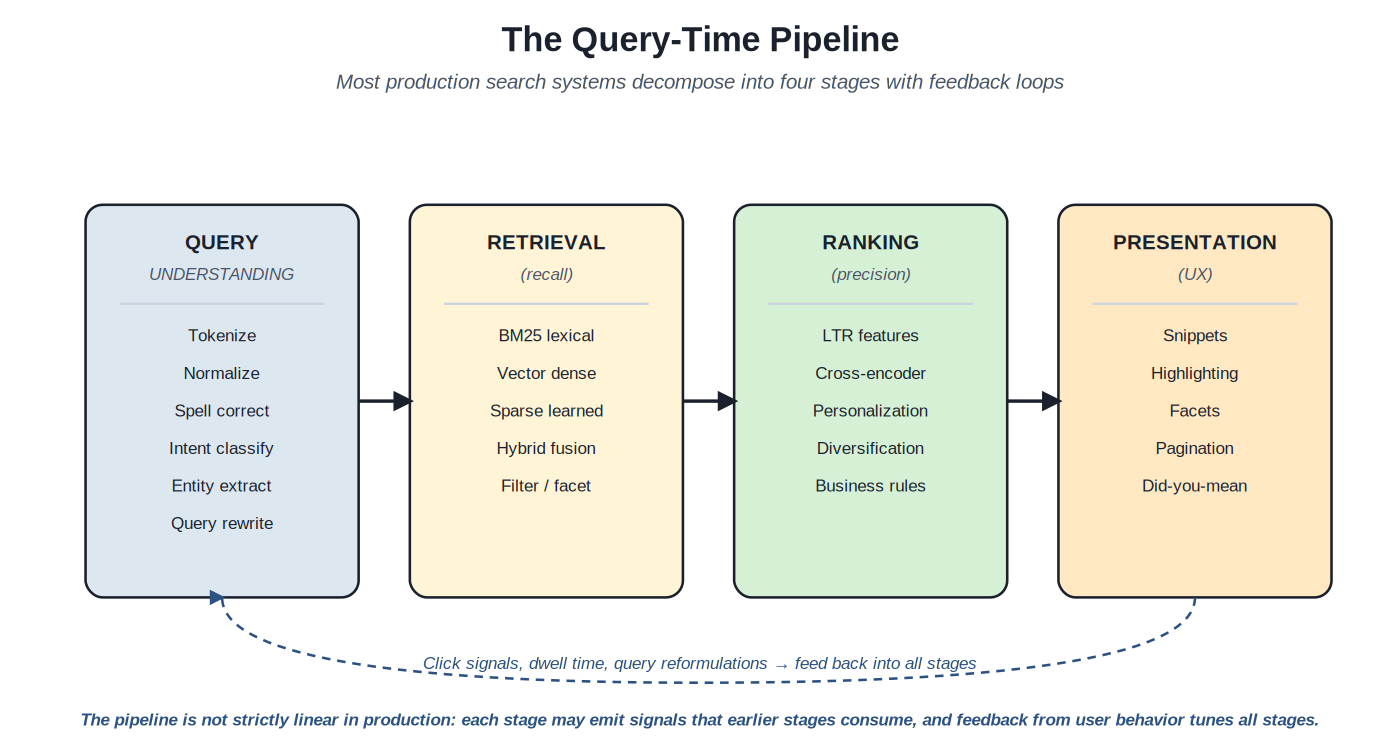
Most production search systems decompose into four stages: query understanding, retrieval, ranking, and presentation. The stages have evolved over thirty years of search practice, with the boundaries between them sharpening as the field has matured. Understanding the pipeline as a structural decomposition — rather than as one monolithic "search" operation — is the prerequisite for understanding everything else in this catalog.
Four stages, with feedback loops. Click signals, dwell time, and query reformulations tune all stages over time.
Query understanding processes the raw user input into a structured representation. Tokenization splits the query into terms. Normalization handles case, accents, and other surface variation. Spell correction handles typos. Intent classification identifies whether this is a navigational, informational, transactional, or conversational query. Entity recognition extracts brands, product types, locations, and other structured signals. Query rewriting handles synonyms, expansions, and known reformulations. The output is a representation the retrieval stage can work with effectively. The future Query Understanding Catalog covers this stage in depth; this volume treats it as a black box that produces structured query signals.
Retrieval finds candidate documents from the indexed corpus. This is the "recall" stage: the goal is to surface documents that might be relevant, with reasonable confidence that anything genuinely relevant is in the candidate set. Retrieval scales to corpora of millions or billions of documents; the constraint is doing so within latency budgets (typically sub-100ms in production) and cost budgets (millions of queries per day at acceptable per-query cost). The patterns in this catalog's Sections A through D cover the major retrieval architectures.
Ranking reorders the candidate set for precision. Where retrieval optimized for recall — finding the right documents — ranking optimizes for getting the right documents to the top. The stage applies expensive scoring methods that wouldn't scale to the full corpus but work fine on a few hundred candidates: learning-to-rank with engineered features, cross-encoder neural rerankers, personalization layers, diversification rules, business-logic boosts. The future Ranking & Relevance Catalog covers this stage in depth; this volume's multi-stage patterns (Section D) document the architectural interaction between retrieval and ranking.
Presentation renders results for the user. Snippets, highlighting, facets, pagination, did-you-mean refinements, zero-results UX. The presentation layer is where search quality becomes user-visible; the upstream stages can be technically excellent and still produce poor user experiences if presentation is wrong. The future Search UX Patterns Catalog covers this stage. The feedback loops from presentation back to all earlier stages — click signals, dwell time, query reformulations, conversion events — are the substrate for online learning, A/B testing, and continuous improvement; the future Search Evaluation Catalog and Search Operations Catalog cover the discipline of using these signals.
The pipeline is not strictly linear in production. Each stage may emit signals that earlier stages consume: a low-confidence retrieval result may trigger query expansion that re-runs retrieval; a personalization signal in ranking may feedback to retrieval as a filter. Feedback from user behavior tunes all stages over time. The architectural patterns documented in this catalog mostly sit within or between specific stages, but the system-level discipline is recognizing the pipeline as a coordinated whole rather than as independent components.
Chapter 2. Retrieval vs. Ranking
The separation between retrieval and ranking is the most important architectural decision in modern search systems. The choice to keep them separate, rather than collapsing both into a single scoring pass, organizes the rest of the architecture. Understanding why the separation works — and what each stage optimizes for — makes most other pattern choices in this catalog easier.
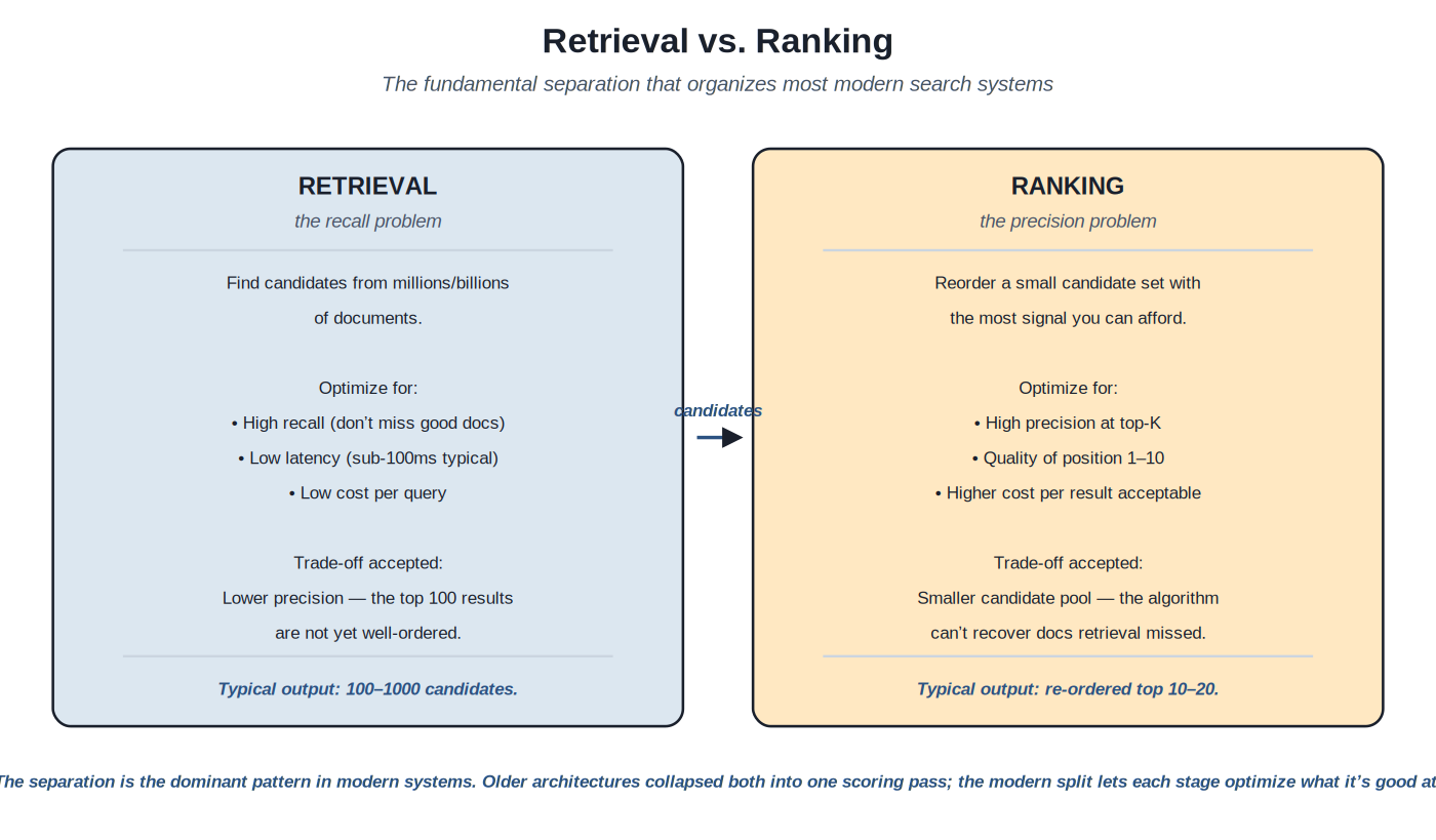
Retrieval optimizes for recall at scale; ranking optimizes for precision on a candidate set. The separation is the dominant pattern.
Retrieval optimizes for recall. The question is: of all the documents in the corpus, which ones might be relevant to this query? The answer needs to come back fast (sub-100ms typical) over very large corpora (millions to billions of documents). The constraint forces simple scoring functions: BM25, vector similarity, sparse-learned scores. These functions are fast enough to compute over the full corpus but don't capture the full picture of what makes a result actually good. The output is a candidate set — typically 100 to 1000 documents — with rough ordering. Anything that isn't in this candidate set has no chance of appearing in the final results; recall at this stage is non-recoverable downstream.
Ranking optimizes for precision. The question is: of these candidates, which order produces the best user experience? The constraint flips: precision matters more than recall (the candidate set is already filtered); per-document scoring cost is acceptable to be much higher (only hundreds of documents, not millions); latency budget is tighter because retrieval already consumed some of the total budget but per-document time is more permissive. The expanded computational budget lets ranking apply expensive methods: learning-to-rank with hundreds of features, cross-encoder neural models that compute query-document attention, personalization layers that integrate user-specific signals, diversification rules that prevent result clustering.
The trade-offs the separation embodies. Retrieval accepts lower precision in exchange for scale; ranking accepts smaller candidate pools in exchange for richer scoring. Together they produce better top-K results than either alone could produce at the system's latency and cost constraints. Collapsing them into one pass forces a single scoring function to handle both jobs, which fails at scale: simple-enough-to-scale scoring is too crude for precision; rich-enough-for-precision scoring is too expensive for scale. The separation is the architecture that resolves the tension.
The historical pattern matters. Search systems in the 1990s and 2000s typically did one-pass scoring. The separation emerged through 2005–2015 as learning-to-rank techniques (Microsoft's RankNet, Yahoo's LambdaMART) demonstrated value but were too expensive to apply at scale. Two-stage architectures became dominant because they let teams use these expensive methods where they paid off (top-K reranking) without paying the cost at scale (full-corpus scoring). By 2026 the separation is the default; single-stage scoring is reserved for specific narrow cases (very small corpora, very simple matching needs).
Chapter 3. The Hybrid Era
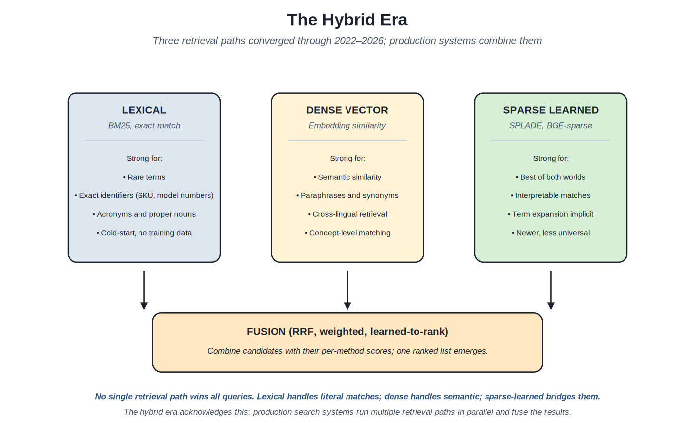
Through 2022–2026, search engineering converged on the recognition that no single retrieval path wins all queries. Lexical retrieval handles literal and identifier-heavy queries that dense retrieval struggles with. Dense vector retrieval handles semantic queries that lexical retrieval misses. Sparse-learned retrieval (SPLADE and successors) bridges the two with interpretable matches and implicit term expansion. Production systems run multiple retrieval paths in parallel and fuse the results.
Lexical, dense, and sparse-learned retrieval converged. Production systems run them in parallel and fuse the results.
Lexical retrieval, anchored in BM25, has been the search industry's workhorse for decades. The pattern handles exact matches with characteristic strengths: rare terms (a query for "ibuprofen" matches documents containing that exact term reliably), exact identifiers (product SKUs, model numbers, error codes), acronyms and proper nouns, cold-start scenarios where no training data is available. The weaknesses are well-known too: synonyms and paraphrases miss ("pain reliever" doesn't match "analgesic" out of the box); concept-level matching requires extensive synonym engineering; cross-lingual retrieval requires translation infrastructure.
Dense vector retrieval emerged through the deep learning era and reached production maturity through 2020–2024. The pattern handles semantic similarity: "pain reliever" and "analgesic" produce similar embeddings even without explicit synonym configuration. Paraphrases, conceptual queries, and cross-lingual retrieval all work better than they do with pure lexical approaches. The weaknesses run in the opposite direction: exact identifier matching is unreliable (the embedding for "SKU-12345" may not specifically privilege documents containing that exact string); cold-start without training data is harder; the embedding model itself is a dependency that needs management and updates.
Sparse-learned retrieval emerged through 2021–2024 as a bridge between the two. SPLADE (Naver Labs, 2021) and similar models produce sparse representations that resemble lexical indexes but with learned term expansion baked in. The pattern preserves the interpretability and exact-match strengths of lexical retrieval while adding semantic expansion. Matches are explainable (which terms triggered the match); rare terms work as in lexical retrieval; semantic expansion happens automatically. The pattern is newer and less universally supported across platforms; it's the third leg of the hybrid stool, increasingly common in 2026 production deployments.
Fusion is where the paths come together. Section C documents the specific patterns: reciprocal rank fusion (RRF) combines ranked lists from multiple paths without requiring score normalization; weighted hybrid scoring combines normalized scores with tunable per-path weights; learned fusion (LTR over the per-path scores) tunes the combination using labeled training data. Each fusion approach has trade-offs in complexity and quality; the right choice depends on whether labeled data is available, whether interpretability matters, and how much per-query latency the fusion adds.
The honest observation about the hybrid era: the era didn't replace lexical retrieval — it added to it. BM25 is alive and well in production search systems alongside dense vector retrieval and sparse-learned approaches. The lexical infrastructure (analyzers, inverted indexes, BM25 scoring) hasn't become obsolete; it's become one path among several. The architectural shift is from "pick one retrieval method" to "run multiple methods in parallel and fuse." The shift is well-established by 2026; production systems that haven't made the transition are typically operating below the working frontier of search quality.
Chapter 4. Multi-Stage Architectures
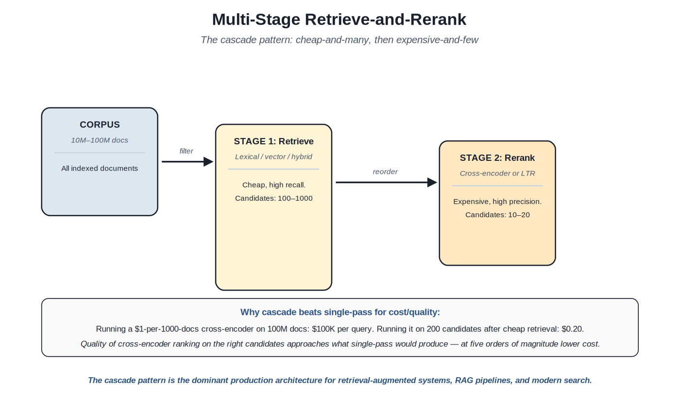
The cascade pattern — cheap-and-many retrieval followed by expensive-and-few reranking — is the dominant production architecture for modern search systems. The pattern emerged from the recognition that the retrieval-ranking separation (Chapter 2) extends naturally into multi-stage cascades, where each stage applies progressively more expensive scoring to progressively smaller candidate sets.
The cascade pattern is the dominant production architecture for retrieval-augmented systems, RAG pipelines, and modern search.
The economic argument is decisive. Running an expensive cross-encoder reranker (millisecond-per-document scoring) on a 100-million-document corpus is computationally impossible at typical query volumes. Running the same cross-encoder on 200 candidates returned by cheap first-stage retrieval is trivially fast. Quality of the cross-encoder ranking on the right candidates approaches what single-pass scoring would produce — at five orders of magnitude lower cost. The cascade pattern is how modern systems get the quality benefits of expensive ranking methods without paying the cost at scale.
The architectural pattern extends to more than two stages in some systems. A three-stage cascade might use: ultra-cheap retrieval (BM25 or simple vector ANN) to produce 10,000 candidates from the full corpus; mid-cost reranking (LTR with engineered features) to reduce to 100 candidates; expensive reranking (cross-encoder neural model) to produce the final top 10–20. Each stage justifies its cost by applying methods that wouldn't scale to the prior stage's candidate count. The trade-off is increased pipeline complexity and per-query latency; the benefit is the ability to apply increasingly sophisticated scoring as the candidate set shrinks.
Quality bounds and recall-precision dynamics. The cascade pattern's quality is bounded by the recall of the cheapest first stage: if relevant documents don't appear in the initial candidate set, no amount of subsequent reranking recovers them. This is why the hybrid era (Chapter 3) matters for the cascade: better first-stage recall through multi-path retrieval produces better cascade output, because the reranker has more good candidates to work with. The cascade and the hybrid patterns are complementary, not competing.
The pattern's prevalence beyond traditional search. RAG (retrieval-augmented generation) pipelines for LLM-based agents use the same cascade architecture: dense or hybrid retrieval against a knowledge base, cross-encoder reranking, top-K documents passed as context to the LLM. The structural pattern is identical; the application changes. Recognizing the cascade in agent retrieval (covered in the agentic AI series, Volume 10) and in classic search is recognizing the same architectural pattern across very different surface applications.
Chapter 5. Query Routing
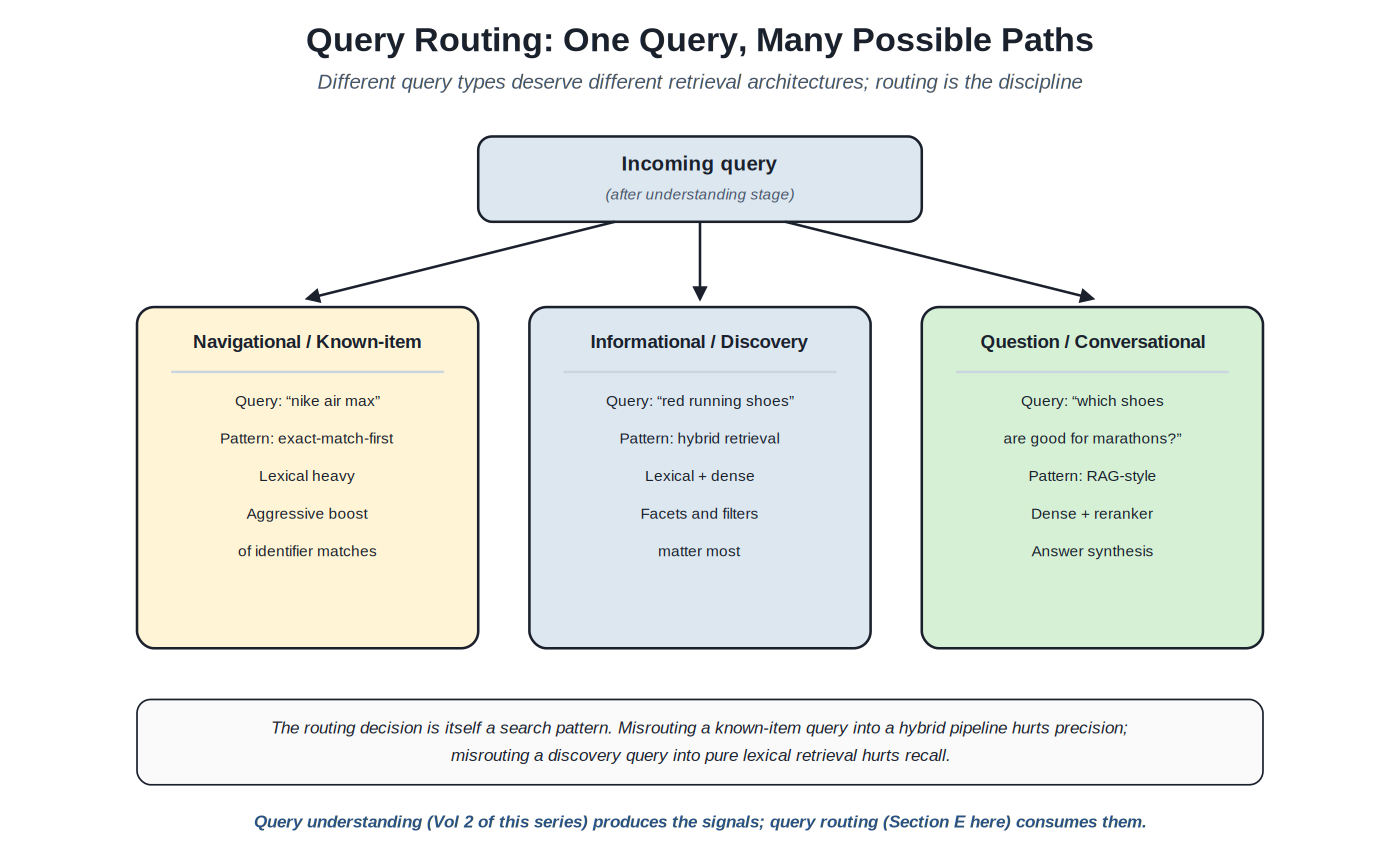
Different queries deserve different retrieval architectures. A navigational query ("nike air max") wants exact-match-first retrieval that surfaces the specific product. An informational query ("red running shoes") wants hybrid retrieval that handles synonyms and related concepts with facets for refinement. A conversational query ("which shoes are good for marathons?") wants RAG-style retrieval with reranking and answer synthesis. Query routing is the discipline of selecting the appropriate architecture for each query type.
One incoming query, multiple possible retrieval paths. The routing decision is itself a search pattern.
The routing decision rests on the output of query understanding. Intent classification produces a signal (navigational vs informational vs conversational vs transactional vs investigational); the router consumes the signal and selects a retrieval path. The router itself can be rule-based (simple heuristics with classifier output as input), classifier-based (an LLM or smaller model that emits routing decisions directly), or learned (a model trained on query/route/outcome triples). Production deployments often combine approaches: rule-based routing for clear cases, classifier-based for ambiguous ones, with learned overlays as data accumulates.
Misrouting has characteristic failure modes. A navigational query routed to a hybrid retrieval pipeline often surfaces semantically-similar-but-wrong products; the user wanted a specific Nike Air Max, got related running shoes. A discovery query routed to pure lexical retrieval misses the synonyms and related concepts that make discovery useful; the user wanted to browse "red running shoes," got only documents containing those exact words and missed equivalents. A conversational query routed to standard retrieval returns a list of links when the user expected a synthesized answer.
The relationship to broader search architecture. Query routing is the connective tissue between query understanding and retrieval architecture; it's where the per-query architectural decisions live. Most of this catalog's patterns are about how to do retrieval well within a specific architectural choice; query routing is the meta-pattern about choosing which architecture to apply. Section E documents the specific routing patterns; the broader principle is that production search systems in 2026 typically have multiple retrieval architectures available and route queries among them, rather than applying one architecture uniformly.
The cost-benefit of routing. Implementing query routing adds complexity: the router itself, multiple retrieval pipelines that need maintenance, evaluation infrastructure for each route, traffic management between routes. The benefit is per-query optimization that uniformly-applied architectures can't produce. The right complexity level depends on the workload's heterogeneity: a search system with mostly one query type may not justify routing; a search system with diverse query types (most e-commerce, most enterprise search, most consumer general-purpose search) typically does. The discipline of routing emerges in production deployments where the cost of one-size-fits-all architectures becomes visible in evaluation data.
Part 2 — The Substrates
Eight sections cover the query-time architectural patterns. Each section opens with a short essay on what its patterns share. Representative patterns appear in the Fowler-style template.
Sections at a glance
- Section A — Lexical retrieval patterns
- Section B — Dense vector retrieval patterns
- Section C — Hybrid retrieval patterns
- Section D — Multi-stage retrieval and reranking
- Section E — Query routing and federation
- Section F — Personalization and context at query time
- Section G — Performance and caching patterns
- Section H — Discovery and resources
Section A — Lexical retrieval patterns
BM25 and the inverted-index foundation that anchors modern search
Lexical retrieval is the foundation of modern search. The inverted index, BM25 scoring, and the analyzer-tokenizer pipeline have been the workhorse architecture for thirty years. The hybrid era (Chapter 3) added paths around lexical retrieval without replacing it. The patterns in this section document the lexical core that production search systems still depend on, often as one path of several in a hybrid pipeline.
BM25 retrieval #
Source: Robertson, Walker, Jones et al., "Okapi at TREC-3" (1995); the foundational lexical scoring function in Elasticsearch, OpenSearch, Solr, and most lexical search engines
Classification — The dominant lexical retrieval pattern — token-based scoring with term frequency and inverse document frequency adjustments.
Retrieve documents based on lexical overlap between query and document, with scoring that accounts for term frequency saturation and document length normalization in a way that produces stable, predictable rankings across heterogeneous corpora.
Pure term-frequency scoring overweights documents that repeat query terms; pure presence-or-absence scoring loses ranking signal. Documents of different lengths get unfair advantages or disadvantages. The simplest scoring functions (TF-IDF) handle the basic case but produce known artifacts: long documents over-rank because they accumulate more term occurrences; documents that mention a query term many times rank artificially high. BM25 addresses these issues with two parameters — k1 (term frequency saturation) and b (length normalization) — that make the scoring stable and tunable across corpora.
The scoring function. For each query term in each candidate document, BM25 computes a score component that combines: term frequency in the document (saturating, so the 10th occurrence adds less score than the 2nd), inverse document frequency (rare terms get higher weight than common ones), and document length normalization (longer documents are penalized relative to the average length). The components multiply per term; per-term scores sum across all query terms.
Parameter tuning. The k1 parameter (typical range 1.2–2.0) controls term frequency saturation: lower k1 means term frequency saturates faster (additional occurrences add less), higher k1 means term frequency continues to add score with each occurrence. The b parameter (typical range 0.5–1.0, default 0.75) controls length normalization: b=1 fully normalizes for length, b=0 ignores length entirely. Defaults work well for many corpora; tuning per corpus can improve quality measurably but requires evaluation infrastructure.
Implementation. BM25 sits on top of an inverted index: a data structure that maps each term to the list of documents containing it (a postings list). Query processing iterates over the query terms, retrieves the postings lists, and accumulates BM25 scores for each candidate document. Top-K candidates are returned. Modern implementations (Lucene, the underlying library of Elasticsearch, OpenSearch, and Solr) optimize this with skipping, early termination, and SIMD instructions.
Variants. BM25F extends BM25 to multi-field documents, allowing per-field weighting (e.g., title weighted higher than body). BM25+ addresses a known weakness with very long documents in certain corpora. BM25L addresses the long-document case differently. These variants are used in specific cases; vanilla BM25 with reasonable parameter tuning handles most production needs.
Strengths and limits. BM25 excels at literal matches, rare terms, and identifier-heavy queries. It produces explainable matches (which terms contributed how much). It scales to billions of documents at sub-100ms latency on modest hardware. It fails at semantic matching (synonyms, paraphrases, conceptual queries) without separate term-expansion or synonym infrastructure. The hybrid era (Chapter 3) addresses these limits by combining BM25 with semantic retrieval rather than replacing BM25.
Almost every production search system as at least one retrieval path. Cold-start systems without labeled training data. Systems with identifier-heavy queries (e-commerce product SKUs, technical documentation with error codes, legal documents with citation patterns). One path within a hybrid retrieval architecture.
Alternatives — dense vector retrieval (Section B) when semantic matching matters and lexical patterns are insufficient. Hybrid retrieval (Section C) for the common case where both semantic and lexical signals matter. Pure vector retrieval is rarely the right answer alone for most production systems; BM25 typically remains one path in the architecture.
- Robertson and Zaragoza, "The Probabilistic Relevance Framework: BM25 and Beyond" (2009)
- Manning, Raghavan, Schütze, Introduction to Information Retrieval (free online, ch. 11)
- Trey Grainger, AI-Powered Search (2024) chapters on lexical foundations
- Elasticsearch / OpenSearch / Solr documentation for production implementations
Code
// Elasticsearch / OpenSearch BM25 query (REST API)
// The default "similarity" for text fields is BM25; this is the canonical match query
GET /products/_search
{
  "query": {
    "multi_match": {
      "query": "running shoes",
      "fields": [
        "title^3", // Boost title 3x (per-field weighting; BM25F-style)
        "description",
        "brand^2"
      ],
      "type": "best_fields"
    }
  },
  "size": 100
}

// To customize BM25 parameters on an index:
PUT /products/_settings
{
  "index": {
    "similarity": {
      "custom_bm25": {
        "type": "BM25",
        "k1": 1.5, // term frequency saturation (default 1.2)
        "b": 0.7 // length normalization (default 0.75)
      }
    }
  }
}

// Solr equivalent (in schema.xml or schema-managed config)
// <similarity class="solr.BM25SimilarityFactory">
// <float name="k1">1.5</float>
// <float name="b">0.7</float>
// </similarity>
Phrase and proximity matching #
Source: Information retrieval foundations; supported natively in Lucene-based engines and Coveo with positional index data
Classification — Pattern for matching multi-term queries as phrases or with position constraints, producing higher precision than bag-of-words BM25.
Boost or restrict matches based on the proximity and ordering of query terms within documents, capturing phrase semantics that bag-of-words scoring loses.
BM25 treats queries as bags of words: "red shoes" and "shoes red" produce identical scoring against documents. Many queries have phrase semantics that should affect ranking: "machine learning" as a phrase is much more specific than "machine" and "learning" separately; "New York" should preferentially match documents about the city rather than documents containing both words in unrelated contexts. Phrase and proximity matching capture these semantics with position-aware scoring.
Phrase queries. Strict phrase matching requires the query terms to appear consecutively in the document. Lucene-based engines support this through positional information in the inverted index: each posting includes the position(s) of the term within the document. The query processor verifies that candidate documents contain the query terms in the specified order at consecutive positions. Phrase queries can be combined with other queries (e.g., must match phrase, should boost on individual terms).
Proximity queries. Relaxed phrase matching allows the query terms to appear within a configurable number of positions of each other ("slop" in Lucene terminology). A slop of 0 is strict phrase matching; slop of 5 allows up to 5 intervening positions; slop of 50 allows the terms to appear anywhere in a reasonably-sized document. Proximity scoring typically boosts matches with smaller distances over matches with larger distances.
Field-specific behavior. Position information is typically maintained per-field; phrase queries operate within a single field. "New York" as a phrase matches title:"New York Times" but not separate occurrences of "New" in title and "York" in body. Production search typically combines per-field phrase matching with cross-field bag-of-words matching for balanced precision and recall.
Span queries. More sophisticated position constraints beyond simple phrase or proximity: "term A within N positions of term B, in either order, both within field C." Span queries support precise positional logic for specific use cases (legal citation matching, technical documentation, structured data extraction). The cost is query complexity and computational overhead; production use is selective.
Boost-not-filter pattern. Phrase and proximity matches are typically used as boost signals rather than as hard filters. A query like "red running shoes" might use phrase matching to boost documents where "running shoes" appears as a phrase while still retrieving documents where the terms appear separately. The pattern preserves recall while improving precision; pure phrase-required queries often produce too few results.
Queries with significant phrase semantics: product names ("iPhone 15 Pro"), proper nouns ("New York Times"), technical terms ("machine learning"), location names ("San Francisco"). E-commerce search where the difference between bag-of-words and phrase matches noticeably affects relevance. Domain-specific search (legal, medical, technical) where multi-word terms carry specific meaning.
Alternatives — dense vector retrieval (Section B) handles phrase semantics implicitly through embedding similarity; it's often used alongside lexical phrase matching in hybrid architectures. Query rewriting (future Query Understanding Catalog) can convert known multi-word terms into atomic tokens that BM25 then handles correctly.
- Lucene documentation on PhraseQuery and SpanQuery
- Elasticsearch / OpenSearch "match_phrase" and "match_phrase_prefix" query documentation
- Coveo phrase boost documentation
Section B — Dense vector retrieval patterns
Embedding similarity and the semantic retrieval paths that emerged through 2020–2026
Dense vector retrieval encodes documents and queries as numeric vectors in a learned embedding space and ranks by similarity. The pattern emerged through the deep learning era and reached production maturity through 2020–2024. By 2026, dense retrieval is a standard component of modern search architectures — typically alongside lexical retrieval (Section C covers the hybrid combination) rather than replacing it.
Dense vector retrieval (HNSW, IVF) #
Source: Malkov and Yashunin, "HNSW" (2016); Jégou et al. on IVF (2011); production implementations in Pinecone, Weaviate, Qdrant, Elasticsearch / OpenSearch (k-NN plugin), Vespa, Vertex AI Vector Search
Classification — Approximate nearest neighbor retrieval over learned embeddings.
Retrieve documents based on semantic similarity by encoding queries and documents into a shared embedding space and finding nearest neighbors in that space, with approximate algorithms that scale to billions of vectors at sub-100ms latency.
Lexical retrieval misses semantic matches. A query for "pain reliever" doesn't match documents about "analgesic" without explicit synonym configuration. Paraphrases ("how do I install Python" vs "python installation guide") require manual query rewriting. Cross-lingual retrieval requires translation infrastructure. Dense vector retrieval addresses these gaps by working in a learned semantic space where conceptually-related terms produce similar vectors regardless of exact lexical overlap.
Embedding generation. A pre-trained or fine-tuned embedding model (sentence-transformers, BGE, E5, OpenAI text-embedding-3, Voyage, Cohere embed) encodes both documents (at index time) and queries (at query time) into dense vectors, typically 384-2048 dimensions. The model is trained so that semantically-similar inputs produce vectors close to each other in the embedding space (typically by cosine similarity or inner product).
Index construction. Dense vectors are stored in a vector index designed for approximate nearest neighbor (ANN) search. HNSW (Hierarchical Navigable Small World) is the dominant algorithm in production: it constructs a layered graph where each node connects to its nearest neighbors at multiple resolution scales, enabling logarithmic-time approximate search. IVF (Inverted File Index) is the alternative: it partitions the vector space into clusters and searches only the clusters closest to the query vector. Different algorithms trade off index size, build time, query latency, and recall accuracy.
Query-time retrieval. The query is encoded into a vector using the same embedding model. The vector index returns approximate K-nearest-neighbors with their similarity scores. The candidates are typically the top 50–500 documents by vector similarity; downstream stages (ranking, reranking) refine the ordering.
Embedding model selection. The choice of embedding model substantially affects retrieval quality. General-purpose models (OpenAI text-embedding-3-large, BGE-large, Voyage 3) work for many use cases. Domain-specific models (legal, medical, code) outperform general models on their domains. Fine-tuned models on domain-specific labeled data outperform off-the-shelf models when training data is available. Model selection is itself a discipline; vendor benchmarks (MTEB, BEIR) provide comparison points but production evaluation on the actual workload is essential.
Production trade-offs. Dense retrieval has higher per-query cost than BM25 (embedding generation at query time, vector index lookup) but the cost is bounded and predictable. Index sizes are larger (1.5KB per 384-dim float32 vector vs. inverted index sizes), though quantization (binary, int8) reduces this. Updates to the corpus require re-embedding affected documents, which has cost; high-update-rate corpora may need batch re-embedding strategies. The model is a dependency that needs versioning and migration management when updated.
Production search where semantic matching matters beyond what synonym engineering provides. RAG pipelines for LLM-based agents (the agentic AI series' Volume 10 covers). Conversational search interfaces. Cross-lingual retrieval. Concept-level search in domains where users naturally use varied vocabulary (consumer search, customer support, knowledge management).
Alternatives — lexical retrieval (Section A) alone for narrow use cases dominated by exact and identifier matches. Hybrid retrieval (Section C) for the dominant production pattern combining both. Sparse-learned retrieval (next entry) as an alternative that preserves some lexical-style interpretability.
- Malkov and Yashunin, "Efficient and robust approximate nearest neighbor search using HNSW" (2018)
- Karpukhin et al., "Dense Passage Retrieval for Open-Domain QA" (2020)
- BEIR benchmark suite (github.com/beir-cellar/beir)
- MTEB leaderboard for embedding model comparison (huggingface.co/spaces/mteb/leaderboard)
Code
// Elasticsearch / OpenSearch k-NN query (using pre-computed query vector)
// Assumes index has a knn_vector field 'embedding' with HNSW configuration
GET /products/_search
{
  "size": 100,
  "query": {
    "knn": {
      "embedding": {
        "vector": [0.012, -0.034, 0.156, ...], // 384-dim query embedding
        "k": 100,
        "num_candidates": 500 // explore more candidates for better recall
      }
    }
  }
}

// Pinecone equivalent
import { Pinecone } from '@pinecone-database/pinecone';
const pc = new Pinecone();
const index = pc.index('products');
const results = await index.query({
vector: queryEmbedding,
topK: 100,
includeMetadata: true
});

// Weaviate equivalent (using nearVector)
const result = await weaviate.graphql.get()
.withClassName('Product')
.withNearVector({ vector: queryEmbedding })
.withLimit(100)
.withFields('title description _additional { distance }')
.do();
Sparse-learned retrieval (SPLADE, BGE-sparse) #
Source: Formal et al., SPLADE (Naver Labs, 2021); BGE-M3 sparse component (BAAI, 2024); production support in Vespa, OpenSearch, custom implementations
Classification — Retrieval pattern combining lexical-style sparse representations with learned term expansion.
Retrieve documents using sparse vector representations — where each dimension corresponds to a vocabulary term — with learned weights that include implicit term expansion, bridging the interpretability of lexical retrieval and the semantic capability of dense retrieval.
Dense vector retrieval is semantically powerful but opaque: it's hard to explain why a specific document matched a specific query, and the embedding space is not directly interpretable. Lexical retrieval is interpretable but limited to exact and configured-synonym matches. Sparse-learned retrieval addresses both: it produces sparse representations (most dimensions zero) that look like extended vocabularies, with learned weights that automatically expand terms based on context. The matches are explainable (which expanded terms triggered the match); semantic capability approaches dense retrieval; the architecture preserves inverted-index efficiency.
Model architecture. A transformer-based model (typically BERT-derived) processes the input text and produces a sparse vector where each dimension corresponds to a token in the model's vocabulary. Most dimensions are zero (the sparsity); non-zero dimensions represent terms the model considers semantically present, including terms not literally in the text. The output for "running shoes" might activate the terms "running" and "shoes" explicitly and also "athletic," "sneakers," "footwear" implicitly with learned weights.
Index construction. Sparse-learned vectors are stored in inverted-index-style structures (since the representations are sparse). The index format resembles a lexical inverted index but with the vocabulary expanded to model token space (~30K terms for BERT-style models) and weighted by the model rather than by BM25 statistics.
Query-time retrieval. The query is processed through the same model to produce a sparse vector. Retrieval is similar to BM25 over the expanded vocabulary: the query's non-zero dimensions are looked up in the inverted index; documents matching multiple query dimensions accumulate scores. The expansion happens at both query and document time, so a query for "pain reliever" may activate "analgesic" and match documents that activated the same term during indexing.
Strengths. Interpretable matches — you can see which terms (including expanded ones) contributed to a match. Implicit term expansion — no manual synonym lists needed. Inverted-index efficiency — the retrieval architecture resembles lexical retrieval rather than vector retrieval. Cold-start without supervised training data — the underlying model is pre-trained.
Limitations. The pattern is newer (post-2021) and less universally supported across platforms than BM25 or dense retrieval. Model dependency creates the same versioning challenges as dense retrieval. The expansion is fixed by the model; it can't be customized at runtime the way explicit synonym lists can. Some platforms (Elasticsearch, OpenSearch) support sparse-learned retrieval through plugins or specific APIs; others (Vespa) support it natively; some (Coveo, Algolia) have varying support as of 2026.
Production search where interpretability of matches matters (e-commerce explaining why a product matched, customer service search where reviewing the match logic matters, regulated domains). Cases where dense retrieval's quality is needed but the opacity is a concern. Workloads with high update rates where the inverted-index-style architecture handles updates more cleanly than dense vector indexes.
Alternatives — dense retrieval (prior entry) when interpretability isn't needed and dense models are stronger for the use case. Hybrid retrieval (Section C) combining sparse-learned with other paths. Pure lexical retrieval for use cases where learned expansion doesn't justify the model dependency.
- Formal et al., "SPLADE: Sparse Lexical and Expansion Model for First Stage Ranking" (2021)
- BAAI BGE-M3 (multi-functionality embedding including sparse output)
- Vespa sparse vector documentation
- OpenSearch neural sparse search documentation
Section C — Hybrid retrieval patterns
Combining lexical and semantic paths through fusion — the dominant modern architecture
The hybrid era (Chapter 3) recognized that no single retrieval path wins all queries. Production systems run lexical, dense, and increasingly sparse-learned retrieval in parallel and fuse the results. Two fusion patterns dominate: Reciprocal Rank Fusion (RRF) for score-normalization-free combination, and weighted hybrid scoring with tunable per-path weights for cases where labeled data supports tuning.
Reciprocal Rank Fusion (RRF) #
Source: Cormack, Clarke, Büttcher, "Reciprocal Rank Fusion outperforms Condorcet and individual rank learning methods" (SIGIR 2009); production support in Elasticsearch / OpenSearch, Vespa, custom implementations
Classification — Fusion pattern combining ranked lists from multiple retrieval methods without requiring score normalization.
Combine ranked results from multiple retrieval methods (lexical, dense, sparse-learned) into a single ranked list, using only the rank positions rather than the raw scores, producing a robust fusion that doesn't require calibration of the underlying scoring functions.
Different retrieval methods produce scores on different scales: BM25 produces unbounded positive scores; cosine similarity produces values in [-1, 1]; SPLADE produces yet another distribution. Combining scores directly requires normalization, and normalization choices substantially affect the fusion quality. Score-based fusion is also sensitive to outliers: a single high-scoring document in one method can dominate the fusion regardless of how the other methods rated it. RRF sidesteps these issues by working only with rank positions, which are inherently bounded and comparable across methods.
The formula. For each document in any of the candidate lists, RRF computes a score: sum over all retrieval methods of 1 / (k + rank_in_that_method), where k is a smoothing constant (typically 60). Documents are sorted by this combined score. Documents that appear high in multiple lists score highest; documents that appear in only one list still get a score but lower; documents not appearing in any list get zero.
Why the formula works. The reciprocal structure (1/rank) gives strong weight to high-ranked positions and small weight to lower positions — matching the intuition that being #1 in one method matters more than being #50. The smoothing constant k prevents the top position from dominating (without k, position 1 would always dominate). The sum across methods combines evidence: documents that multiple methods agree on get boosted; documents that only one method liked get included but ranked lower.
Robustness. RRF's robustness to score scales and outliers makes it the default fusion choice when adding new retrieval methods. A team running BM25-only retrieval can add dense retrieval and combine via RRF without re-tuning anything; the addition either improves results (the dense retrieval found good documents BM25 missed) or has negligible effect (the dense retrieval found the same documents). The pattern is hard to make worse with bad input — a poorly-tuned retrieval method that adds noise tends to add documents at low rank positions, where they affect the fusion minimally.
Parameters. The k parameter (smoothing constant) is the main tunable. Lower k (e.g., 10) gives more weight to top-ranked documents and is more sensitive to position differences. Higher k (e.g., 100) makes the fusion more uniform across positions. The default k=60 from the original paper works well empirically; tuning makes marginal differences in most workloads.
Limitations. RRF doesn't use score magnitudes — a document at rank 5 with high score and a document at rank 5 with low score are treated identically. When the underlying retrieval methods produce well-calibrated, comparable scores, score-based fusion can outperform RRF. RRF also doesn't learn from training data; weighted or learned fusion can exploit labeled data when available. In practice, RRF is the right default; teams move to more sophisticated fusion when they have the evaluation infrastructure to verify improvement.
Adding a new retrieval method to an existing pipeline (dense alongside BM25, sparse-learned alongside dense). Hybrid retrieval where score normalization is uncertain or unavailable. Cases where labeled training data isn't available for learning a fusion. Production deployments where simplicity and robustness matter more than peak quality optimization.
Alternatives — weighted hybrid (next entry) when labeled data and tuning infrastructure are available. Learning-to-rank over per-method scores when the team has sufficient training data and infrastructure for LTR. Pure single-method retrieval for narrow use cases where one method clearly dominates.
- Cormack et al., "Reciprocal Rank Fusion outperforms Condorcet and individual rank learning methods" (2009)
- Elasticsearch / OpenSearch RRF documentation ("rrf" rank fusion)
- Vespa rank-fusion documentation
Code
// Elasticsearch / OpenSearch RRF combining BM25 and dense vector retrieval
GET /products/_search
{
  "retriever": {
    "rrf": {
      "retrievers": [
        {
          "standard": {
            "query": {
              "match": { "title": "running shoes" }
            }
          }
        },
        {
          "knn": {
            "field": "embedding",
            "query_vector": [0.012, -0.034, ...],
            "k": 100,
            "num_candidates": 500
          }
        }
      ],
      "rank_window_size": 100,
      "rank_constant": 60 // k parameter; default 60
    }
  },
  "size": 50
}

// Manual RRF implementation (for platforms without native support):
function reciprocalRankFusion(rankedLists, k = 60) {
const scores = new Map();
for (const list of rankedLists) {
list.forEach((docId, rank) => {
// rank is 0-indexed; RRF uses 1-indexed positions
const contribution = 1 / (k + rank + 1);
scores.set(docId, (scores.get(docId) || 0) + contribution);
});
}
return [...scores.entries()]
.sort((a, b) => b[1] - a[1])
.map(([docId, score]) => ({ docId, score }));
}
Weighted hybrid scoring #
Source: Search engineering practitioner literature; production patterns across Coveo, Vespa, Algolia, custom implementations
Classification — Fusion pattern combining per-path scores with tunable weights, typically after normalization.
Combine scores from multiple retrieval methods using explicit per-method weights, supporting per-query-type tuning and integration with learned ranking models that need calibrated combined scores.
RRF (prior entry) is robust but doesn't use score magnitudes. When the underlying retrieval methods produce useful score information — not just rank order, but how confident each method is — score-based fusion can outperform RRF. The challenge is normalizing scores across methods with different scales, and choosing weights that produce good results. Weighted hybrid scoring handles this through explicit normalization and tunable weights, at the cost of more configuration than RRF requires.
Score normalization. Each retrieval method's scores are normalized to a common scale, typically [0, 1]. Min-max normalization (per-query, using the min and max scores in the candidate set) is common; z-score normalization (using the distribution mean and standard deviation) is an alternative. Normalization is per-query rather than global because score distributions vary substantially across queries.
Weighted combination. The fused score for a document is a weighted sum of its normalized scores from each method: score = w_lexical \ lexical_norm + w_dense \ dense_norm + w_sparse * sparse_norm. Weights are typically tuned via evaluation against labeled data, A/B testing, or learning-to-rank approaches that treat the per-method scores as features.
Per-query-type weighting. Different query types deserve different fusion weights. Navigational queries ("SKU-12345") typically weight lexical higher; informational/discovery queries weight dense higher; conversational queries weight dense plus reranking higher. Production systems may have multiple weight profiles selected by query routing (Section E).
Documents not in all lists. A document may appear in some retrieval methods' candidate sets but not others. The pattern handles this with explicit decisions: missing scores can be treated as zero (the document gets no contribution from that method but isn't penalized further); or as a small penalty (the document is slightly disfavored relative to documents that all methods returned). The choice affects ranking and should be tuned.
Comparison with RRF. Weighted hybrid scoring can outperform RRF when: (1) the per-method scores carry useful magnitude information beyond rank order; (2) labeled training data is available for tuning weights; (3) per-query-type tuning is feasible. RRF tends to outperform weighted hybrid when the underlying scores are poorly calibrated, when training data is limited, or when simplicity and operational robustness matter more than peak optimization.
Mature search deployments with labeled training data and evaluation infrastructure. Per-query-type optimization where different query types deserve different weights. Cases where the underlying retrieval methods produce well-calibrated, meaningful scores. Integration with learning-to-rank pipelines where per-method scores feed downstream LTR models.
Alternatives — RRF (prior entry) for simpler deployments or when tuning data isn't available. Learning-to-rank over per-method scores when sufficient training data and infrastructure support the more complex approach.
- Search engineering practitioner literature on hybrid retrieval tuning
- Vespa rank profile documentation (supports weighted multi-phase ranking natively)
- Coveo machine learning ranking documentation
Section D — Multi-stage retrieval and reranking
The cascade pattern — cheap-and-many followed by expensive-and-few
Multi-stage retrieval extends the retrieval-ranking separation (Chapter 2) into explicit cascades. The first stage retrieves candidates at scale using cheap scoring; subsequent stages rerank progressively smaller candidate sets with progressively more expensive methods. The pattern is the dominant production architecture for modern search and for RAG pipelines in agentic AI systems.
Two-stage retrieve-and-rerank #
Source: Industry-standard architecture, anchored in learning-to-rank literature (Liu, "Learning to Rank for Information Retrieval," 2009) and modern neural reranking practice
Classification — The dominant production search architecture: a fast retrieval stage produces candidates; a slower ranking stage reorders them.
Apply expensive ranking methods (LTR, cross-encoder rerankers, personalization) to a small candidate set produced by cheap first-stage retrieval, achieving better top-K quality than single-stage scoring at acceptable cost.
Single-stage scoring forces a difficult trade-off: scoring functions cheap enough to apply to the full corpus are too crude for high-precision ranking; scoring functions rich enough for precision are too expensive to apply to the full corpus. The two-stage pattern resolves this by using each stage for what it's good at: fast first-stage retrieval scales to billions of documents and produces good candidate recall; slower second-stage ranking applies expensive methods to 100–1000 candidates and produces good top-K precision. The decoupling lets both stages optimize their own constraints.
Stage 1 — retrieval. Cheap scoring methods (BM25, vector similarity, hybrid via RRF) run over the full corpus and produce a candidate set, typically 100–1000 documents. The stage optimizes for recall: anything genuinely relevant should appear in this set, even if not in its final correct order. Latency budget is typically 30–80ms; cost per query is whatever the cheap method costs.
Stage 2 — reranking. Expensive scoring methods (LTR models with hundreds of engineered features, cross-encoder neural rerankers, personalization layers, business-logic boosts) reorder the candidate set. The stage optimizes for top-K precision: positions 1–10 should be the best documents in the candidate set in the most useful order. Latency budget is typically 20–100ms; cost per query is the expensive scoring method's cost times the candidate count.
Stage boundary tuning. The number of candidates returned by stage 1 (the cutoff K) is a tunable parameter. Smaller K (e.g., 100) means stage 2 is cheaper but stage 2 has fewer candidates to choose from — missing the right document in stage 1 can't be recovered. Larger K (e.g., 1000) means stage 2 sees more candidates and can produce better top-K results, but stage 2 cost grows proportionally. Production deployments tune K based on the marginal quality improvement of larger candidate sets against the marginal cost.
Evaluation across stages. Each stage should be evaluated separately. Stage 1 is evaluated for recall at K (is the right document in the top K candidates); stage 2 is evaluated for top-K metrics (NDCG, MAP) given the candidate set. Stage 1 quality bounds the system's overall quality; stage 2 quality determines how well the system exploits stage 1's output. Confusing the two during evaluation leads to misdiagnosed quality issues.
Beyond two stages. Three-stage and four-stage cascades exist in production systems: ultra-cheap retrieval (e.g., BM25 alone) to 10,000 candidates, mid-cost reranking (LTR) to 100 candidates, expensive reranking (cross-encoder) to top 10–20. Each stage justifies its computational cost by applying methods that wouldn't scale to the prior stage's candidate count. Marginal benefit of additional stages diminishes; most production systems run two or three stages.
Almost every production search system above toy scale. The pattern is the default; single-stage scoring is reserved for narrow cases (very small corpora, very simple matching needs, latency-critical applications where the second stage's cost is unacceptable). Modern RAG pipelines for LLM-based agents use the same architecture.
Alternatives — single-stage scoring for narrow specialized cases. The multi-stage pattern is so universal that justifying single-stage requires specific reasons (latency constraints, corpus size, simplicity needs).
- Liu, "Learning to Rank for Information Retrieval" (2009) for LTR foundations
- Nogueira and Cho, "Passage Re-ranking with BERT" (2019) for neural reranker introduction
- Reimers and Gurevych, sentence-transformers cross-encoder documentation
Cross-encoder reranking #
Source: Sentence-Transformers cross-encoder models; commercial rerankers (Cohere Rerank, Voyage Rerank); open models (BGE Reranker, mxbai-rerank)
Classification — Reranking pattern using transformer models that jointly process query and document for high-precision scoring.
Apply joint query-document attention to rank candidate documents with much higher precision than independent embedding similarity, accepting higher per-document cost in exchange for better top-K quality.
Dense vector retrieval (Section B) encodes queries and documents independently into embeddings, then computes similarity. The independence is what makes retrieval scalable — documents can be embedded offline and indexed; only the query needs embedding at query time. But the independence is also a limitation: the model never sees query and document together, so it can't capture interactions specific to that pair. Cross-encoders address this by jointly processing query and document, capturing fine-grained interaction signals that bi-encoders (dense retrieval) miss — at the cost of being too expensive to apply at retrieval scale.
Model architecture. A transformer (typically BERT-derived, or larger modern variants) takes the query and a candidate document as a single concatenated input. The model's attention layers process both jointly, computing fine-grained interactions: which query terms match which document terms, how the document's overall context affects each match, contextual signals that bi-encoders can't capture. The output is a single relevance score for that query-document pair.
The bi-encoder vs cross-encoder trade-off. A bi-encoder encodes query and document independently; the similarity is a single dot-product or cosine computation per pair, and document embeddings can be pre-computed. A cross-encoder requires the full transformer forward-pass per pair, which is hundreds to thousands of times more expensive but captures interactions the bi-encoder misses. Bi-encoders scale to billions of documents at retrieval time; cross-encoders are limited to hundreds of candidates per query.
Production deployment. Cross-encoders run as reranking stages after first-stage retrieval (Section A, B, or C). Typical configuration: retrieve 100–500 candidates with cheap methods; rerank with cross-encoder to produce final top 10–20. Latency per query depends on candidate count and model size; production systems target sub-100ms reranking budgets with batched scoring on accelerated hardware.
Model options. Open models (BGE Reranker, mxbai-rerank, sentence-transformers cross-encoders) are free and self-hostable but require infrastructure. Commercial APIs (Cohere Rerank, Voyage Rerank, Mixedbread Rerank) provide reranking as a service; latency is the network round-trip plus inference time, cost is per-document scored. Trade-offs are similar to the broader self-host vs API decision in the agentic AI series.
Fine-tuning. Cross-encoders can be fine-tuned on domain-specific labeled data (relevance judgments, click data, hard negatives mined from production). Fine-tuned models typically outperform off-the-shelf models on the domain they were tuned for. The discipline of cross-encoder fine-tuning is itself a specialty within search engineering; the relevance & ranking volume (planned future volume) would cover the methodology.
Production search where top-K precision matters and the cost of expensive reranking is justified by quality gains. RAG pipelines for agents where the documents passed to the LLM matter substantially. High-stakes search (legal, medical, customer service) where wrong top results have meaningful costs. Cases where first-stage retrieval quality is good but the ordering needs refinement.
Alternatives — LTR-based reranking with engineered features for cases where labeled training data is rich and feature engineering is feasible. Pure first-stage retrieval for low-stakes applications where rerank cost isn't justified. Multi-stage cascades that put cross-encoders even later (as a third stage after LTR reranking) for very high-quality requirements.
- Nogueira and Cho, "Passage Re-ranking with BERT" (2019)
- Sentence-Transformers cross-encoder documentation (sbert.net)
- Cohere Rerank documentation (cohere.com/rerank)
- BGE Reranker (huggingface.co/BAAI/bge-reranker-v2-m3)
Section E — Query routing and federation
Selecting retrieval architecture per query; combining results across multiple indexes
Query routing (Chapter 5) is the discipline of selecting which retrieval architecture to apply to each query. Federation is the related but distinct discipline of combining results across multiple separate indexes — different content types, different shards, different specialized stores. The patterns in this section document how production systems handle the heterogeneity that uniform single-index single-architecture deployments can't address.
Intent-based query routing #
Source: Practitioner pattern across e-commerce search (Bass Pro Shops, Best Buy, Coveo deployments); enterprise search platforms; documented in Grainger's AI-Powered Search
Classification — Pattern for selecting retrieval architecture based on query intent classification.
Route each incoming query to the most appropriate retrieval pipeline based on classified intent (navigational, informational, conversational, transactional), producing better per-query results than uniformly applying one architecture.
Queries vary substantially in what retrieval they need. A navigational query ("nike air max") wants exact-match retrieval that surfaces the specific known item. An informational query ("red running shoes") wants hybrid retrieval with facets for refinement. A conversational query ("which shoes are good for marathons?") wants RAG-style retrieval with reranking and possibly answer synthesis. A transactional query ("buy nike air max 270 size 10") wants filter-heavy retrieval. Applying one uniform architecture to all of these compromises every category.
Intent signal source. Intent classification (covered in the future Query Understanding Catalog) produces the routing signal. The classifier may be rule-based (length, structure, keyword patterns), classifier-based (a small LLM or trained model that outputs intent), or learned (a model trained on query/intent labels). Production deployments often combine: rule-based for clear cases, classifier-based for ambiguous cases.
Route definitions. Each intent maps to a retrieval architecture. Navigational → lexical-heavy with aggressive exact-match boosting. Informational → hybrid retrieval with facet generation. Conversational → dense retrieval with cross-encoder reranking. Transactional → filter-applied retrieval with structured constraint handling. The mappings are implemented as separate retrieval pipelines that the router selects among.
Confidence-based fallback. The router's intent classification has confidence scores. High-confidence classifications route directly to the designated pipeline. Low-confidence classifications can: run multiple pipelines in parallel and fuse the results (defensive routing); route to a default "general" pipeline (conservative routing); or use the broadest architecture (recall-preserving routing). The choice affects quality and cost.
Per-route tuning. Each retrieval pipeline can be tuned independently. The navigational pipeline's BM25 parameters, exact-match boosts, and facet handling are tuned for known-item queries. The informational pipeline's hybrid weights are tuned for discovery queries. Per-route tuning is a substantial advantage over uniform architectures, where any tuning is a compromise across query types.
Operational complexity. Routing adds infrastructure: the router itself, multiple retrieval pipelines, evaluation per route, monitoring and alerting per route, deployment management for multiple pipelines. The complexity is justified when the workload's heterogeneity is significant; deployments with mostly one query type often don't justify routing.
Monitoring and analytics. Per-route metrics (latency, recall, click-through, conversion) reveal whether routing is working. Misrouted queries appear as anomalies: high-CTR queries in the wrong pipeline; low-CTR queries that should have been routed differently. The discipline of monitoring routing decisions is itself a search operations pattern; the future Search Operations Catalog covers it.
E-commerce search with mixed query types (navigational, informational, transactional). Enterprise search with diverse content types and use cases. Consumer search platforms where the query distribution spans many intents. Cases where evaluation data shows that one-size-fits-all retrieval produces visibly worse results for specific query types.
Alternatives — single-architecture deployment for narrow workloads with uniform query types. Federated multi-index retrieval (next entry) for cases where content heterogeneity matters more than query heterogeneity. Per-query hybrid weighting (Section C) for lighter customization without full routing infrastructure.
- Trey Grainger, AI-Powered Search, chapters on query understanding and routing
- Coveo machine learning query intent documentation
- Practitioner case studies (Bass Pro Shops, Best Buy, etc.) on e-commerce search routing
Federated multi-index search #
Source: Established pattern in enterprise search; production deployments across Elasticsearch / OpenSearch (cross-cluster search), Solr (distributed search), Coveo (federation), Vertex AI Search, Azure AI Search
Classification — Pattern for combining results from multiple separate indexes into a single result set.
Search across multiple separate indexes — different content types, different domains, different geographical or organizational boundaries — and combine the results into a coherent unified response, with appropriate ranking across the sources.
Many production systems have content in multiple separate indexes for legitimate reasons: different content types (products vs articles vs videos vs support tickets) with different schemas; different domains with different update patterns; different regions or organizations with different governance; legacy indexes that can't be merged. Single-index queries don't work; the user shouldn't have to choose which index to search. Federated search addresses this by routing queries to multiple indexes and combining results, presenting the unified view as if it were a single index.
Query distribution. The federation layer takes the incoming query and distributes it to relevant indexes. Distribution can be: broadcast (send to all indexes; combine all results); routed (send only to indexes likely to have relevant content based on query analysis); progressive (start with high-priority indexes, add others if needed). Each strategy trades latency and cost for completeness.
Per-index processing. Each index processes the query using its appropriate retrieval pipeline. Different indexes may use different architectures: the products index uses hybrid retrieval; the articles index uses BM25 plus dense retrieval; the videos index uses metadata-only lexical retrieval. The federation layer doesn't require uniformity across indexes; each can optimize independently.
Result combination. Results from multiple indexes are combined into a single ranked list. The challenge: scores from different indexes aren't directly comparable. Solutions include: per-source result blocks ("Products (5), Articles (3), Videos (2)") avoiding the combination problem entirely; rank-based fusion (RRF) treating each index as a retrieval method; learned ranking models that take per-source scores plus features as input. The choice affects UX as much as quality.
Latency management. Federated search's latency is bounded by the slowest index involved (when results from all indexes are needed for fusion). Production patterns: timeout per index with partial results if slow indexes don't return in time; asynchronous federation where slower indexes contribute results that appear later in the UX; pre-fetching for high-priority indexes. The patterns prevent slow indexes from degrading user experience.
Per-source diversity. Some federated UX shows results grouped by source (the per-source result block pattern). Others show one merged ranked list. The merged pattern is more demanding (requires score comparison across indexes) but produces a more unified experience. The grouped pattern is easier to implement and clearer about provenance, but may be less useful when users don't care which index a result came from.
Enterprise search across multiple content repositories (Confluence + SharePoint + Drive + Jira + Slack + custom systems). Large e-commerce with multiple content types (products + articles + brand pages + community content). Multi-region deployments where content sovereignty requires separate indexes. Multi-tenant SaaS with per-tenant indexes plus shared content.
Alternatives — unified single-index deployment when content can be normalized and combined; the operational complexity of multiple indexes is usually only justified when single-index isn't feasible. Intent-based routing (prior entry) when query heterogeneity matters more than content heterogeneity.
- Elasticsearch / OpenSearch cross-cluster search documentation
- Solr distributed search and cross-collection documentation
- Coveo federation and source documentation
- Glean and Hebbia documentation on federated enterprise search architectures
Section F — Personalization and context at query time
Injecting user, session, and contextual signals into retrieval
Personalization at query time adjusts retrieval based on signals beyond the query string: who the user is, what they've done before, where they are, what time it is, what device they're on. The patterns range from minimal (locale-based result filtering) to extensive (full per-user re-ranking). The discipline involves choosing the right level of personalization for the use case — too little misses easy wins, too much produces opacity, filter bubbles, and operational complexity.
User and session context injection #
Source: Established pattern across e-commerce, enterprise search, consumer search; documented in Tunkelang's writing on personalized search and Grainger's AI-Powered Search
Classification — Pattern for incorporating user-specific and session-specific signals into retrieval and ranking.
Adjust retrieval and ranking based on signals available at query time — user history, current session context, locale, device, time of day — to produce results more relevant to the specific user in the specific context than results based on the query string alone.
Two users entering the same query string may want different results. A returning customer searching "running shoes" wants results filtered or boosted based on their prior purchases (size, brand affinity, price tier). A user in a specific geographic region wants results adjusted for local availability. A user with prior session context (just viewed a specific brand) probably wants related items boosted. Pure query-based retrieval misses all of these signals; personalization integrates them.
Signal sources. User signals: long-term profile (preferences, history, demographics where available). Session signals: recent activity in the current session (viewed items, applied filters, prior queries). Contextual signals: locale, device type, time, day of week, page from which the search was triggered. Operational signals: A/B test cohort, feature flags, business context (current promotions, inventory).
Integration patterns. Signals can be injected at different pipeline stages. At retrieval: signals become filter conditions (locale restricts inventory) or boost factors (preferred brands boost candidates). At ranking: signals become features for LTR models or inputs to learned rerankers. At result post-processing: signals affect diversification, business-rule application, result presentation. Different signals fit different stages; multi-stage signal use is common in production.
Privacy and opacity considerations. Personalization that affects results without user awareness can be problematic. Best practice: keep personalization signals visible ("Recommended based on your recent activity"), allow opt-out, log the signals used for any specific result. The discipline overlaps with the agentic AI series' compliance and UX volumes; in search specifically, personalization opacity erodes user trust over time.
Cold-start handling. New users without history, anonymous sessions, no available locale: personalization needs to degrade gracefully. The pattern: fall back to general retrieval; use weak available signals (IP-based locale, device-type defaults) cautiously; let user feedback (clicks, dwells) build the personalization signal over the session.
Operational complexity. Personalization adds infrastructure: user profile storage, session state management, signal extraction at query time, feature engineering for ranking models, evaluation that accounts for per-user effects. The complexity is justified when personalization meaningfully improves outcomes; for narrow use cases where one-size-fits-all retrieval works, personalization is over-engineering.
Filter bubbles and diversity. Aggressive personalization can collapse results to a narrow set the user has previously engaged with, missing valuable discovery. Production patterns include diversification rules that limit how much personalization narrows results, exploration injection that surfaces non-personalized candidates, and periodic re-evaluation that catches when personalization is hurting outcomes.
E-commerce search where user history and preferences meaningfully affect what users want. Enterprise search where user role, team, and access patterns affect relevance. Consumer search where session context (current task, prior queries) shapes intent. Multi-region deployments where locale-based personalization is mandatory.
Alternatives — non-personalized retrieval for narrow use cases or for cold-start situations. Privacy-preserving alternatives (on-device personalization, federated approaches) for regulated or privacy-sensitive deployments. The right level of personalization depends on the use case; defaulting to maximum personalization is typically wrong.
- Daniel Tunkelang's writing on personalized search and ranking
- Trey Grainger, AI-Powered Search, chapters on personalization
- Coveo personalization documentation
- Algolia personalization documentation
Section G — Performance and caching patterns
Result caching and query optimization for latency and cost
Search workloads have characteristic patterns that caching exploits: queries repeat (the long tail of unique queries plus a heavy head of popular queries); result sets are stable for most queries (the underlying corpus changes slower than the query rate); some operations are deterministic and cacheable (analyzer output, embedding generation for known text). Caching strategies tuned to these patterns produce substantial latency and cost reductions.
Query result caching strategies #
Source: Established pattern in production search; documented across Elasticsearch / OpenSearch (request cache, query cache), Solr (filter cache, query result cache), Coveo (result cache), Vespa, Algolia
Classification — Patterns for caching query results, intermediate computations, and analyzer outputs.
Reduce query latency and infrastructure cost by caching results at appropriate granularity: full result sets, intermediate retrieval candidates, filter results, analyzer outputs, embedding computations.
Production search has heavy query repetition. A small head of popular queries can drive 30–60% of total query volume; the same queries produce the same results until the underlying corpus changes. Computing these results from scratch on every request wastes compute. Caching repeated results substantially reduces both per-query latency (cache hits return in microseconds vs. milliseconds for full retrieval) and infrastructure cost (popular queries' results computed once and served many times).
Result-level caching. The full ranked result list for a query is cached. Cache key includes the query string and any parameters that affect results (filters, sort, user/session context if personalized). Cache invalidation triggers on corpus updates: when documents change, affected cached entries must be invalidated. The pattern works well for non-personalized queries with stable corpora; personalization and frequent updates reduce hit rates.
Filter result caching. Filter queries (e.g., "status:active AND category:shoes") often repeat with different free-text queries. Caching the document-set produced by the filter (typically as a bitset or roaring bitmap) lets subsequent queries combine the filter result with their text query quickly. Solr's filter cache is the canonical implementation; similar mechanisms exist in Elasticsearch and others.
Analyzer and tokenization caching. Analyzers (tokenization, normalization, stemming) produce deterministic output for given input. Caching the analyzed form of common terms avoids redundant analyzer runs. The pattern has small per-operation savings but at scale becomes meaningful.
Embedding caching. For dense retrieval (Section B), query embeddings are generated at query time. Caching embeddings for common queries avoids redundant embedding model calls; embedding generation can be a substantial fraction of dense retrieval latency. Cache TTL depends on whether the embedding model itself updates.
Cache invalidation challenges. The fundamental difficulty of caching: knowing when cached data is stale. Approaches: TTL-based (entries expire after fixed time; simple but stale data is served until expiry); event-based (cache invalidated on corpus updates; more precise but requires invalidation infrastructure); version-based (cache key includes corpus version; works for batch update patterns). Production systems typically combine TTLs with event-based invalidation for important changes.
Cache architecture. In-process caches (each search node has its own cache) are simple but produce duplication and cold-start issues on each node. Shared caches (Redis, Memcached) reduce duplication but add network latency. Hybrid patterns (small in-process L1 cache plus larger shared L2 cache) balance the trade-offs. The right architecture depends on cluster size and query patterns.
Production search above modest scale where query repetition produces meaningful cache hit rates. Use cases with stable corpora where invalidation overhead is manageable. Latency-sensitive applications where cache hits provide noticeable user experience improvements. Cost-sensitive deployments where infrastructure savings from caching are material.
Alternatives — no caching for highly personalized retrieval where cache hit rates are low. No caching for high-write-rate corpora where invalidation overhead exceeds caching benefits. Selective caching (filter caches only; result caches only for non-personalized queries) for mixed workloads.
- Elasticsearch / OpenSearch request cache and query cache documentation
- Solr filter cache and query result cache documentation
- Coveo result cache documentation
- Algolia caching documentation
Section H — Discovery and resources
Where to track search engineering discipline as the field continues to evolve
Search engineering has thirty-plus years of accumulated literature, but the discipline continues to evolve: the hybrid era through 2022–2026, sparse-learned retrieval through 2021–2024, increasingly capable reranking models, the cross-pollination with agentic AI through RAG. Staying current requires tracking multiple sources — academic literature, practitioner books, vendor documentation, the conferences where the discipline's practitioners gather.
Search engineering communities and references #
Source: Multiple academic, practitioner, and vendor sources
Classification — Resources for staying current on search engineering as the discipline evolves.
Provide pointers to the active sources of search engineering knowledge across academic research, practitioner literature, vendor documentation, and community gatherings.
Search engineering is a deep, well-established discipline but with active research and practice frontiers. New retrieval methods, new reranking models, new fusion approaches, new platform features emerge continuously. Production teams need ongoing tracking to keep their architectures current.
Foundational texts. Manning, Raghavan, Schütze, Introduction to Information Retrieval (free online at nlp.stanford.edu/IR-book) remains the canonical IR textbook. Trey Grainger's AI-Powered Search (Manning, 2024) covers the modern hybrid era extensively. Doug Turnbull and John Berryman, Relevant Search (Manning, 2016) covers practical relevance engineering for lexical search.
Academic conferences. SIGIR (ACM Special Interest Group on Information Retrieval) is the premier IR conference; annual proceedings cover the state of the research frontier. WSDM (Web Search and Data Mining) and ECIR (European Conference on Information Retrieval) are adjacent venues. Papers from these venues filter into production typically 2–5 years after publication; tracking the venues catches innovations early.
Industry conferences. Haystack (haystackconf.com) is the leading practitioner conference for search relevance engineering, organized by OpenSource Connections. Berlin Buzzwords covers search and data alongside related topics. AI-Powered Search Conference (related to Grainger's book) covers the modern hybrid era. ApacheCon includes Lucene/Solr tracks.
Practitioner writing. Daniel Tunkelang (dtunkelang.medium.com) writes on search and personalization. OpenSource Connections (opensourceconnections.com) publishes practitioner content on Solr, Elasticsearch, and broader relevance engineering. Vendor blogs (Elastic, OpenSearch, Solr/Lucidworks, Coveo, Algolia, Pinecone, Vespa) cover platform-specific patterns and capabilities.
Communication channels. Relevancy Engineering Slack (organized by OpenSource Connections) is the primary practitioner community. Reddit communities (r/searchengines, r/elasticsearch) for casual discussion. LinkedIn search engineering groups for professional context. Conference attendance produces network effects that the asynchronous channels can't replicate.
Evaluation benchmarks. BEIR (github.com/beir-cellar/beir) is the canonical retrieval benchmark suite with multiple datasets. MTEB (huggingface.co/spaces/mteb/leaderboard) covers embedding model evaluation. MS MARCO is the canonical web search dataset for training and evaluation. Tracking benchmark leaderboards reveals which methods are improving and which have plateaued.
Teams building or maintaining production search systems. Engineers transitioning into search from adjacent fields (data engineering, ML engineering, application development). Continuous education as the discipline evolves. Reference when specific patterns prove insufficient in practice.
Alternatives — outsourced consulting (firms like OpenSource Connections, RelevantSearch.AI, etc.) for high-stakes engagements where in-house expertise development isn't the right investment. Internal pattern documentation for teams with mature practice. The combination of external tracking and internal knowledge is the working pattern for most production search teams.
- Manning, Raghavan, Schütze, Introduction to Information Retrieval (free online)
- Trey Grainger, AI-Powered Search (Manning, 2024)
- Doug Turnbull and John Berryman, Relevant Search (Manning, 2016)
- Haystack Conference (haystackconf.com); Berlin Buzzwords (berlinbuzzwords.de)
- BEIR benchmark suite (github.com/beir-cellar/beir)
- MTEB leaderboard (huggingface.co/spaces/mteb/leaderboard)
- Relevancy Engineering Slack (search-relevance.slack.com via OSC invitation)
Appendix A — Pattern Reference Table
Cross-reference of the search patterns covered in this volume, what each provides, and when to use each.
| Pattern | Provides | When to use | Section |
|---|---|---|---|
| BM25 retrieval | Lexical scoring | Default first-stage retrieval | Section A |
| Phrase and proximity | Multi-word semantics | Queries with phrase meaning | Section A |
| Dense vector retrieval | Semantic similarity | Semantic matching needs | Section B |
| Sparse-learned (SPLADE) | Lexical + expansion | Interpretable semantic match | Section B |
| Reciprocal Rank Fusion | Robust hybrid combination | Adding new retrieval paths | Section C |
| Weighted hybrid scoring | Tuned combination | Mature systems with labels | Section C |
| Two-stage retrieve-rerank | Cost–quality balance | Almost all production systems | Section D |
| Cross-encoder reranking | High-precision top-K | When precision matters | Section D |
| Intent-based routing | Per-query architecture | Heterogeneous workloads | Section E |
| Federated multi-index | Multi-source results | Cross-repository search | Section E |
| User context injection | Personalized results | User-specific relevance | Section F |
| Query result caching | Latency / cost savings | Repeated query patterns | Section G |
Appendix B — The Planned Search Engineering Series
This catalog is intended as Volume 1 of a series targeting seven to nine volumes. The planned scope:
- Volume 1 — The Search Patterns Catalog (this volume) — query-time architectural patterns.
- Volume 2 — The Query Understanding Catalog — tokenization, normalization, spell correction, intent classification, entity recognition, query rewriting, synonyms.
- Volume 3 — The Indexing and Document Engineering Catalog — analyzers, field design, enrichment pipelines, chunking, embedding strategies, document normalization.
- Volume 4 — The Ranking and Relevance Catalog — BM25 variants, vector similarity, hybrid scoring, learning-to-rank (LambdaMART, neural rerankers), feature engineering.
- Volume 5 — The Search Evaluation Catalog — NDCG, MAP, MRR, judgment collection, A/B testing methodology, regression detection.
- Volume 6 — The Search Operations Catalog — relevance tuning workflows, query log analysis, zero-result and low-CTR detection, judgment list maintenance.
- Volume 7 — The Search UX Patterns Catalog — autocomplete, facets and filters, snippets, did-you-mean, zero-results UX, personalization surfaces.
- Volume 8 — The Search Platforms Survey — Elasticsearch, OpenSearch, Solr, Coveo, Algolia, Vespa, Vertex AI Search, Typesense, with architectural positioning.
- Volume 9 (optional) — The Semantic and Vector Search Catalog — deeper treatment of embedding model selection, ANN index choice, reranking model selection.
The target of seven to nine volumes is deliberate. Search engineering has accumulated enough discipline to fill many more volumes, but the value proposition is durable structural reference — not exhaustive coverage. Existing books (Grainger, Turnbull, Manning et al.) provide comprehensive coverage; the catalog's contribution is the Fowler-style format applied to the field. More than nine volumes risks sprawl in a domain already well-covered by other literature.
Appendix C — Relationship to the Agentic AI Catalog Series
This catalog runs parallel to a seventeen-volume catalog of agentic AI architecture, sharing format, visual style, and methodology. The two series interact at specific points where the disciplines overlap, and they share a perspective on what catalog-grade structural reference can offer.
Where the disciplines overlap. Multi-stage retrieval (Section D of this volume) is the same architectural pattern as RAG retrieval in agentic AI systems (Volume 10 of that series). Dense vector retrieval (Section B here) is foundational to RAG. Cross-encoder reranking (Section D here) is increasingly part of production RAG pipelines. The shared structural patterns are recognized in both series; the surface applications differ but the underlying architecture is identical.
Where the disciplines diverge. Agentic AI emphasizes LLM-as-the-substrate; search engineering emphasizes retrieval-as-the-substrate. Agent workflows are about coordinating LLM calls with tools and memory; search workflows are about retrieving and ranking documents for users. The catalogs address different practitioner audiences (AI engineers and search engineers respectively) even when they cover overlapping technical patterns. Reading both series gives the practitioner the structural vocabulary for both disciplines; reading one is sufficient for practitioners focused on that side.
Where the methodologies align. Both series use the Fowler-style pattern format. Both treat structural vocabulary as more durable than specific products. Both include perishable products-survey volumes (one in the agentic series; one planned for the search series). Both maintain the discipline of stopping — the agentic series declined to extend past seventeen volumes despite candidates being available; the search series targets seven to nine and should hold to that target.
The two catalogs together cover the structural vocabulary of two adjacent practitioner disciplines. The agentic AI side is younger and more provisional; the search engineering side is older and more stable. Where they overlap, the catalogs reinforce each other; where they diverge, they cover different practitioner needs without redundancy.
Appendix D — Discovery and Standards
Resources for tracking search engineering discipline:
- Foundational texts: Manning et al., Introduction to Information Retrieval; Grainger, AI-Powered Search; Turnbull and Berryman, Relevant Search.
- Academic conferences: SIGIR, WSDM, ECIR for the research frontier.
- Industry conferences: Haystack (relevance engineering), Berlin Buzzwords, ApacheCon (Lucene/Solr).
- Practitioner writing: Daniel Tunkelang on search and personalization; OpenSource Connections on relevance engineering; vendor blogs (Elastic, OpenSearch, Solr/Lucidworks, Coveo, Algolia, Pinecone, Vespa).
- Communities: Relevancy Engineering Slack (via OpenSource Connections); Reddit r/elasticsearch, r/searchengines.
- Benchmarks: BEIR for retrieval, MTEB for embedding models, MS MARCO for web search.
- Open-source projects: Lucene/Solr, Elasticsearch/OpenSearch, Vespa, Qdrant, Weaviate as both implementations to study and communities to engage with.
Two practical recommendations. First, attend Haystack Conference if possible — the practitioner network it produces is unmatched in the field. Second, BEIR is the closest thing to an objective comparison point for retrieval methods; tracking BEIR leaderboards informs which methods are improving relative to others. These two anchors orient most other ongoing learning.
Appendix E — Omissions
This catalog covers about 12 patterns across 8 sections — the scope of a structural volume on query-time architectures. The wider search engineering discipline includes much that isn't covered here:
- Query understanding patterns in depth (tokenization, normalization, spell correction, intent classification, entity recognition). Planned Volume 2.
- Indexing and document engineering. Planned Volume 3.
- Learning-to-rank methodology, feature engineering, training pipelines. Planned Volume 4.
- Search evaluation methodology (NDCG, MAP, MRR, judgment collection, A/B testing). Planned Volume 5.
- Search UX patterns (autocomplete, facets, snippets). Planned Volume 7.
- Specific platform comparisons (Elastic vs OpenSearch vs Solr vs Coveo vs Algolia). Planned Volume 8.
- Semantic and vector search beyond the patterns here. Planned Volume 9 if the series extends that far.
- Search at very large scale (Google, Bing, web-scale challenges). Outside this catalog's scope; specialized literature exists.
- Search in specialized domains (legal, medical, scientific, code search) beyond passing mention. Each domain has its own literature.
- Multimodal search (image + text, video understanding) beyond brief reference. Emerging discipline deserving its own treatment if it stabilizes.
Appendix F — On Starting a Parallel Series
This is Volume 1 of a new catalog series running parallel to the agentic AI series. Starting a second series rather than extending the first reflects a deliberate choice about scope and audience. The agentic AI series covers practitioners building with LLMs and agents; the search engineering series covers practitioners building search systems. The disciplines overlap substantially — modern search uses dense retrieval, modern agents use RAG — but the audiences differ in their primary focus and the practitioner communities they participate in.
The parallel-series structure has trade-offs. Two series mean more total maintenance burden than one would, and they require keeping the boundaries clear so readers know which to engage. The benefit: each series can be sized appropriately for its discipline. Agentic AI needed seventeen volumes to cover its still-emerging structural vocabulary; search engineering should need seven to nine because its vocabulary is more stable. Forcing search into the agentic series would have compromised both; the parallel structure lets each be sized correctly.
The format transfer is the easy part. The Fowler-style entry template, the diagrammatic style, the structural vocabulary discipline, the deliberate stopping — all transfer from one series to the other without modification. The harder discipline is keeping the search series focused on durable structural vocabulary rather than letting it drift into exhaustive coverage of a well-studied field. The agentic series faced the opposite challenge: its field was still emerging, so the risk was capturing provisional patterns as if they were durable. The search series' challenge is the opposite: with thirty years of accumulated content available, the discipline is selecting what's genuinely structural rather than recreating what existing books already cover.
Volume 1 of the search series is the foundation for the rest. The patterns documented here — retrieval-ranking separation, the hybrid era, multi-stage cascades, query routing — are the structural vocabulary that subsequent volumes assume. Volume 2 (Query Understanding) feeds into the routing patterns documented in Section E. Volume 4 (Ranking and Relevance) extends the reranking patterns documented in Section D. Volume 5 (Evaluation) provides the methodology for tuning the patterns this volume documents. Each subsequent volume can be read independently, but the structural vocabulary established here grounds all of them.
Whether the series continues to its planned seven to nine volumes is the same question the agentic series faced. The discipline of stopping applies here too. If subsequent volumes don't clear the bar of genuine structural contribution, they shouldn't be written. The catalog's value rests on each volume earning its place; producing volumes for the sake of completeness erodes the value proposition. The agentic series ended at seventeen volumes with explicit acknowledgment that the bar should keep rising; the search series should hold to its smaller target with the same discipline.
— End of The Search Patterns Catalog —
— Volume 1 of the Planned Search Engineering Series —