The Ranking and Relevance Catalog
The mathematics of ordering: BM25 variants, vector similarity, hybrid fusion, learning-to-rank, cross-encoders, calibration.
About This Catalog
This is Volume 4 of the Search Engineering Series, covering ranking and relevance — the discipline of ordering candidate documents to maximize the quality of top-K results. Where Volume 1 documented the architectural patterns that produce candidate sets (lexical retrieval, dense retrieval, hybrid fusion, cascade architectures) and Volume 5 documented the evaluation methods that measure ranking quality, this volume sits in between: the methods, features, and techniques that determine what order the candidates appear in once they've been retrieved.
Ranking is the densest, most specialized discipline in the search series. The accumulated practitioner knowledge spans twenty-five years — from hand-tuned BM25 boost configurations in the early 2000s, through pairwise and listwise learning-to-rank in 2005-2015, to neural rerankers and LLM-based ranking through 2020-2026. The methods don't replace each other; they compose into cascades, with each era contributing to a specific stage of the production pipeline. This volume catalogues the methods at each layer and the patterns that make them productive.
The volume's perspective. Ranking quality determines search quality. Retrieval can find the right candidates, evaluation can measure outcomes, but ranking is what actually determines what users see and click. A search system with mediocre retrieval and excellent ranking outperforms one with excellent retrieval and mediocre ranking. The investment in ranking methods, features, and infrastructure typically produces the largest quality returns of any single area of search engineering investment.
Scope
Coverage:
- Scoring function patterns: BM25 and its variants in production depth, vector similarity scoring, hybrid score combination.
- Learning to Rank: pointwise, pairwise, and listwise loss functions; gradient-boosted decision tree models (LambdaMART, XGBoost ranking, LightGBM ranking); neural LTR.
- Feature engineering: the four feature categories, feature pipelines, feature stores, the discipline of feature selection.
- Neural rerankers: cross-encoder architectures, late-interaction models (ColBERT family), LLM-as-reranker patterns.
- Personalization in ranking: user features, session features, contextual signals.
- Diversification and result quality: MMR, similar-result avoidance, intent diversity.
- Multi-objective ranking: balancing relevance, freshness, diversity, business rules in a single ranking pipeline.
Out of scope (covered in other volumes):
- Query-time architectural patterns (cascade architecture, hybrid retrieval, query routing). Volume 1 covers.
- Query understanding (tokenization, normalization, intent classification, entity recognition). Planned Volume 2.
- Indexing and document engineering (analyzers, field design, embedding strategies). Planned Volume 3.
- Evaluation methodology (metrics, judgment collection, online testing). Volume 5 covers.
- Day-to-day tuning operations and query log analysis. Planned Volume 6.
- Search UX patterns. Planned Volume 7.
How to read this catalog
Part 1 ("The Narratives") is conceptual orientation: the ranking discipline as a whole; the learning-to-rank evolution from pre-2005 hand-tuned scoring through 2026 neural rerankers; feature engineering as the foundation of ranking quality; neural rerankers in production cascades; the multi-objective nature of production ranking where relevance is one objective among several. Five diagrams sit in Part 1.
Part 2 ("The Substrates") is the pattern reference, organized by section. Each section opens with a short essay on what its patterns share. Representative patterns appear in the Fowler-style template with concrete code examples for the central methods.
Part 1 — The Narratives
Five short essays orient the reader to ranking as engineering discipline. The reference entries in Part 2 assume the vocabulary established here.
Chapter 1. The Ranking Discipline
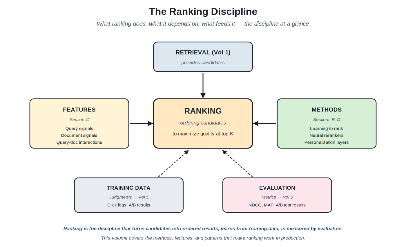
Ranking is the subdiscipline of search engineering that determines result order. Retrieval (Volume 1) produces candidates; evaluation (Volume 5) measures quality; ranking is what actually orders the candidates to produce the result list users see. The discipline encompasses scoring functions, learned models, feature engineering, neural reranking architectures, personalization layers, diversification rules, and the multi-objective balancing that production ranking always involves.
Ranking sits between retrieval (provides candidates) and evaluation (measures quality), depending on features and methods to do its work.
The discipline's position in the broader search pipeline. Retrieval finds candidates fast at scale; ranking refines the candidate ordering with more expensive methods that wouldn't scale to the full corpus. The retrieval-ranking separation (Volume 1 Chapter 2) is the architectural foundation that lets each stage optimize its own constraints. Ranking gets a small candidate set (typically 100–1000 documents) and a richer computational budget than retrieval had; it spends that budget on methods that wouldn't work at full-corpus scale but produce substantially better top-K ordering on the candidate set.
What ranking depends on. Features: per-query signals, per-document signals, query-document interactions, contextual signals. Methods: scoring functions, learned models (LTR), neural rerankers. Training data: relevance judgments and click logs from the evaluation infrastructure Volume 5 covers. Evaluation: the metrics and methods Volume 5 documents tell you whether your ranking changes helped. The dependencies make ranking a connector discipline: ranking work intersects with retrieval architecture, feature engineering, model training, evaluation, and production operations. Improvements in any of the dependencies enable better ranking; weaknesses in any of them constrain ranking quality.
Where ranking complexity comes from. The discipline has more accumulated technical depth than most other parts of search engineering. The reason: ranking is where the per-query work happens, where the per-document scoring happens, where the per-pair interactions matter. The combinatorial space is huge — hundreds of features times thousands of candidates times millions of queries — and the methods for navigating it have evolved over twenty-five years through multiple paradigm shifts. The depth means ranking has more specialized expertise than other subdisciplines; ranking engineers exist as a recognized role at major search companies where retrieval engineers and evaluation engineers don't always.
The role of business outcomes. Academic ranking research measures relevance with NDCG and similar metrics. Production ranking serves business outcomes: revenue, conversion, satisfaction, productivity. The gap between academic and business goals is real — a system that improves NDCG by 5% may improve conversion by 1%, or by nothing, depending on which queries improved and how. Production ranking discipline integrates the academic methods with business outcome measurement (Volume 5 Section G); the multi-objective ranking patterns documented in this volume's Section G capture the integration.
Chapter 2. The Learning-to-Rank Evolution
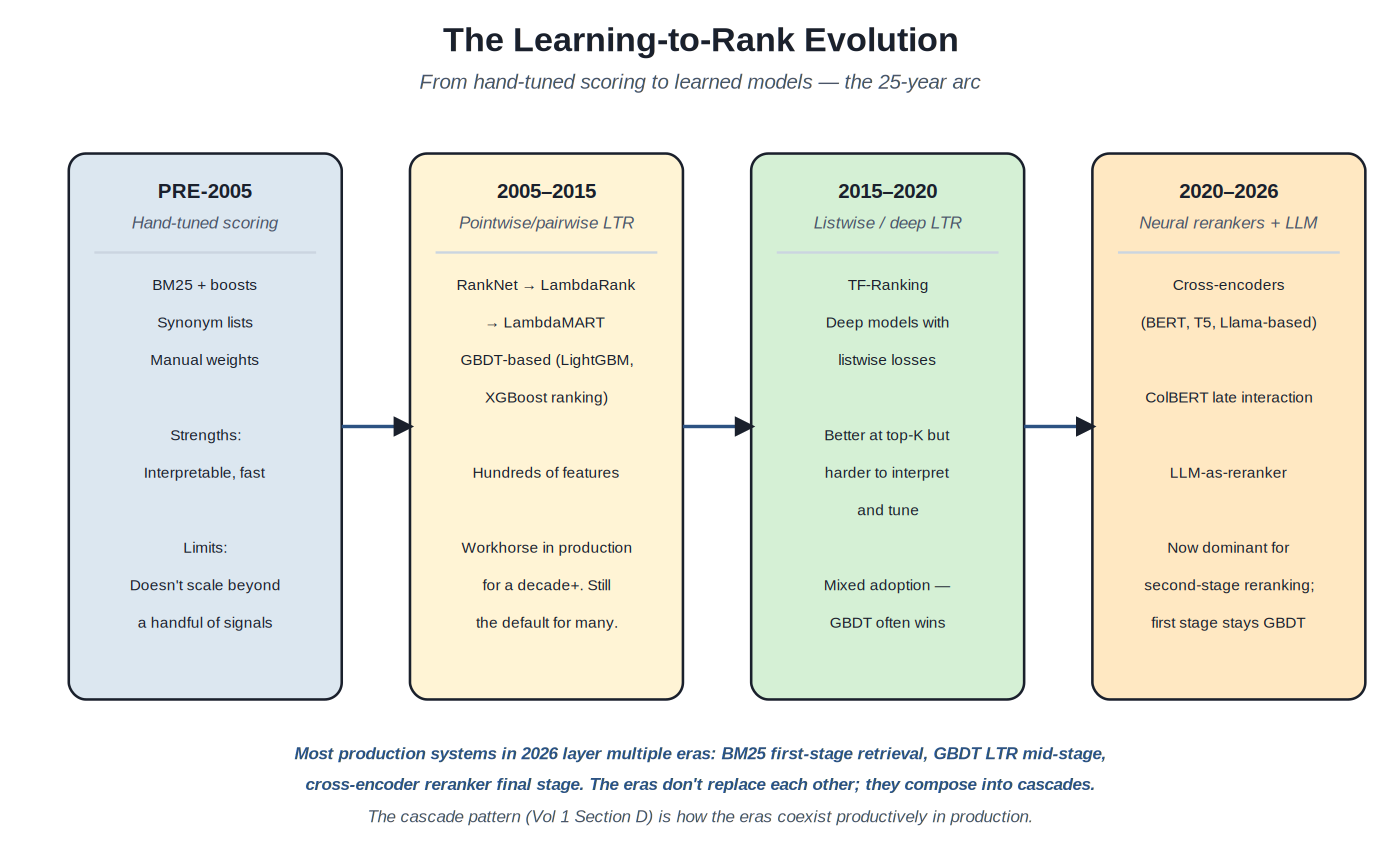
Ranking methodology has evolved through four broad eras, each adding capabilities the previous era couldn't handle but not replacing it entirely. Production systems in 2026 typically use methods from multiple eras in a cascade. Understanding the evolution as a sequence of additions — rather than as replacements — is the framework for understanding why production ranking architectures look the way they do.
Four eras of ranking methodology. The eras compose in production cascades; they don't replace each other.
Pre-2005: hand-tuned scoring. Before learning to rank was practical, ranking was BM25 (Volume 1 Section A) plus hand-tuned boosts: weights on specific fields, synonym lists, query-specific overrides for important queries. Search engineers tuned these by hand based on evaluation results and intuition. The methods scale to a handful of signals and a modest number of queries; beyond that, the manual tuning becomes intractable. Hand-tuned scoring is still the baseline for cold-start systems and the foundation that LTR builds on top of.
2005–2015: pointwise and pairwise LTR. Microsoft Research's RankNet (Burges et al., 2005), then LambdaRank (2006), then LambdaMART (2010) introduced gradient-boosted decision trees as the dominant LTR method. The breakthrough: instead of learning per-document relevance scores (pointwise) or per-pair preferences (pairwise) separately, the LambdaMART loss combined preference signals with metric-aware gradients (the "lambda" in the name) to directly optimize ranking metrics. GBDT-based LTR with implementations in LightGBM and XGBoost remained the production workhorse for over a decade; many production systems in 2026 still use it as their primary ranking method, often as a mid-stage between retrieval and neural reranking.
2015–2020: listwise and deep LTR. The transition from pointwise/pairwise to listwise loss functions was substantial methodologically but produced mixed adoption results. TF-Ranking (Google's open-source library) provided production-grade listwise LTR with TensorFlow; deep listwise models could in principle outperform GBDT on top-K metrics. In practice, GBDT often remained competitive on most workloads, and the additional complexity of deep listwise models wasn't always justified. The era contributed important methodology (listwise losses, deep architectures for ranking) but didn't produce wholesale replacement of GBDT in production.
2020–2026: neural rerankers and LLM-based ranking. The cross-encoder revolution (BERT-based, then T5-based, then Llama-based rerankers) changed the calculation: jointly encoded query-document pairs produce substantially better top-K rankings than independent encoding plus learned scoring. The cost is computational — 100–1000x more expensive per pair than GBDT inference — but bounded because rerankers operate on small candidate sets (top 100–500 from retrieval). Late-interaction models (ColBERT) reduce the cost while preserving most of the quality. LLM-as-reranker (Cohere Rerank, Voyage, BGE Reranker, monoT5, RankZephyr) is now the dominant pattern for high-quality top-K reranking. First-stage retrieval and mid-stage GBDT typically remain; the neural reranker is added as a final stage.
The cascade as historical synthesis. The production pattern in 2026 layers all four eras: BM25 for first-stage retrieval (pre-2005 methodology, still optimal for cheap recall); hybrid retrieval with vector similarity (post-2020 methodology, complements lexical); GBDT LTR for mid-stage refinement (2005–2015 methodology, still excellent value per dollar); neural cross-encoder for final-stage reranking (2020–2026 methodology, where quality matters most). Each era contributes to the layer where its methods are most cost-effective. The cascade (Volume 1 Section D) is the architecture that makes this composition productive.
Chapter 3. Feature Engineering for Ranking
Features are where ranking quality is made or lost. The choice of features for an LTR model has more impact on quality than the choice of LTR algorithm itself; a model with great features and decent algorithm typically outperforms a model with weak features and excellent algorithm. Feature engineering for ranking is its own substantial discipline, with characteristic categories and patterns that this section introduces.
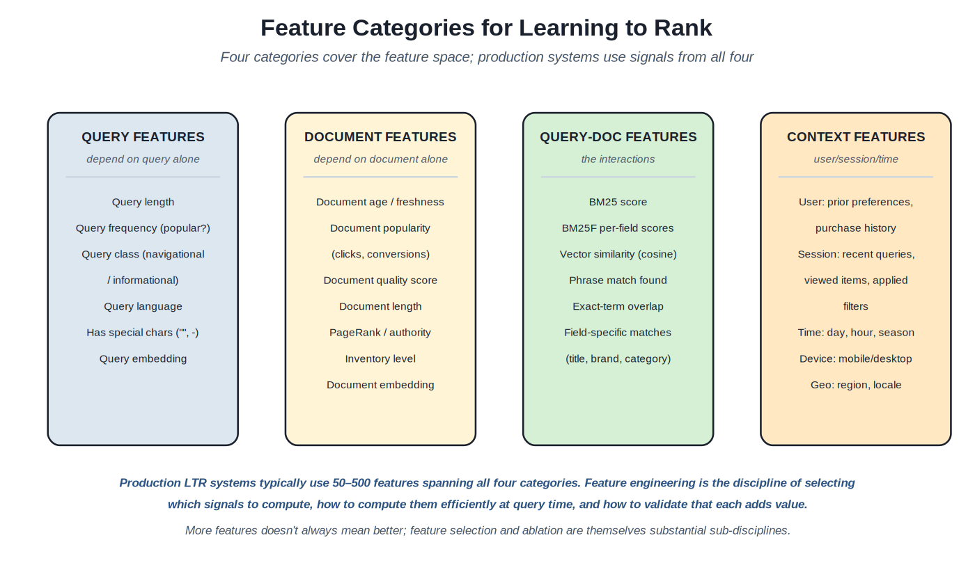
Four feature categories cover the production feature space. Each category has characteristic signals and engineering patterns.
Query features depend only on the query. Length (number of tokens), frequency (how often the query has been seen in production), classification (navigational / informational / conversational / transactional from query understanding, Volume 2), language, character composition (contains numbers, special characters, quoted phrases). Query features capture properties of what the user is asking; they help the model adapt its scoring based on what kind of question it's answering. A model that handles long discovery queries and short navigational queries equally without distinguishing them produces compromised results on both; query features let the model differentiate.
Document features depend only on the document. Age (how recently published or updated), popularity (clicks, views, conversions over time windows), authority signals (PageRank for web search; brand authority for e-commerce; citation count for academic), inventory level (for commerce: in-stock, low-stock, sold-out), quality scores (content quality assessments, completeness metrics), embeddings (dense vector representations from Section B). Document features capture intrinsic properties of candidates; they support the model in distinguishing high-quality documents from lower-quality ones regardless of query.
Query-document features are the interactions. BM25 score is the canonical example: it's the lexical match score between this specific query and this specific document. BM25F per-field scores break this down further (title match, body match, brand match). Vector similarity between query embedding and document embedding. Phrase match indicators (the query's exact phrase appears in the document). Term overlap statistics (what fraction of query tokens appear in the document). Field-specific signals (the query term appeared in the title field; the query term appeared in the brand field). Query-document features are typically the most informative for ranking; they capture the relevance signal that the model must combine with other signals.
Context features capture user, session, time, and environment. User features: prior preferences derived from purchase history, viewing history, demographic signals where available. Session features: queries earlier in the session, items viewed, filters applied. Time features: hour of day, day of week, seasonal indicators. Device features: mobile vs desktop, browser, app version. Geographic features: region, locale, inferred latitude/longitude. Context features enable personalization (Section E) and contextual adaptation that the model would miss with only query, document, and query-document features.
Feature engineering patterns. Production teams typically work with 50–500 features in mature LTR systems. Adding features without ablation is the most common mistake: a feature that looks plausible may add noise rather than signal; ablation studies (train with and without the feature, measure metric change) reveal which features genuinely contribute. Feature pipelines compute features at training time and query time; the pipelines must produce identical features in both contexts (training-serving skew is a major production failure mode). Feature stores (Feast, Tecton, and similar platforms) provide infrastructure for managing this; many production teams build custom feature pipelines optimized for their specific use case.
Chapter 4. Neural Rerankers in Production
The neural reranker era (2020–2026) produced the largest single quality improvement in modern search ranking. Cross-encoder architectures — jointly encoding query and document into a single transformer model — substantially outperform independent encoding on top-K precision. The cost is computational: cross-encoders are 100–1000x more expensive per pair than bi-encoder similarity. The cascade pattern (Volume 1 Section D) is how production systems integrate cross-encoders without paying their cost at retrieval scale.
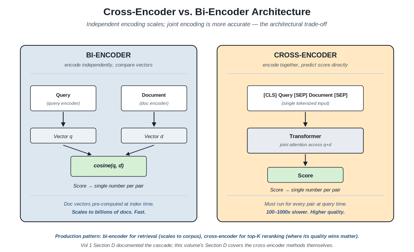
Bi-encoders scale to the full corpus by encoding independently; cross-encoders sacrifice that scalability for joint attention quality.
Why cross-encoders win on quality. A bi-encoder produces query and document embeddings independently, then computes similarity (cosine or dot product). The independence is what makes retrieval scalable — document embeddings precomputed at index time, only the query needs encoding at query time. But the independence means the model never sees the query and document together; it can't capture fine-grained interactions specific to the pair. A cross-encoder concatenates query and document and processes them jointly through a transformer; the attention layers compute query-aware document representations and document-aware query representations simultaneously. The joint attention captures interactions the bi-encoder misses: which query terms matter in this document, how the document's overall context affects each match, contextual signals that independent encoding can't represent.
Why cross-encoders can't replace bi-encoders. A cross-encoder must run for every query-document pair at query time. Pre-computing scores isn't possible because the query is unknown until the user issues it. For a corpus of 100M documents, running a cross-encoder on every document for every query is computationally impossible at production volumes. The cost is bounded only when the cross-encoder operates on a small candidate set: top-K from retrieval (typically K = 100 to 1000). On 200 candidates, cross-encoder reranking takes 50–200ms on accelerated hardware; on 100M candidates it would take days per query.
Production cross-encoder patterns. The cascade architecture (Volume 1 Section D): retrieval produces candidates (BM25 or hybrid), then cross-encoder reranks. Latency is bounded by total candidate count times per-pair scoring time; production deployments tune the candidate count for the latency budget. Hardware matters: GPUs accelerate transformer inference substantially over CPUs; the choice of accelerator affects throughput and cost. Batching matters: scoring multiple candidates in parallel via batched inference is much more efficient than serial scoring. Production deployments typically batch 8–64 candidates per inference call depending on model size and hardware.
Cross-encoder options. Open models: sentence-transformers cross-encoders (free, self-hostable, smaller and faster), BGE Reranker (BAAI, strong quality / cost trade-off), mxbai-rerank, monoT5 (text-to-text reranking), RankZephyr (open instruction-tuned reranker). Commercial APIs: Cohere Rerank (cohere.com, easy integration), Voyage Rerank (voyage AI), Mixedbread Rerank. Each has trade-offs in quality, latency, cost, and operational model; the agentic AI series' Volume 16 covers the self-host vs API question generally.
Late-interaction models. ColBERT (Khattab and Zaharia, 2020) and its successors (ColBERTv2, PLAID) introduced a middle path: compute per-token document embeddings at index time, then at query time compute per-token query embeddings and combine with documents via a learned interaction. The model is more expensive than bi-encoder but cheaper than cross-encoder; quality is between the two, often closer to cross-encoder than to bi-encoder. Late-interaction is used in production deployments where the cross-encoder cost is too high but bi-encoder quality is insufficient; the architectural complexity is non-trivial, so adoption is selective.
Chapter 5. Multi-Objective Ranking
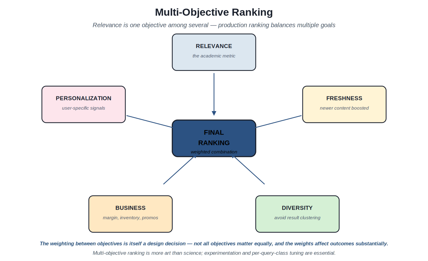
Production ranking serves multiple objectives simultaneously. Relevance to the query is the central one, but freshness (newer content), diversity (avoiding result clustering), personalization (user-specific signals), and business rules (margin, inventory, promotions, brand priorities) all factor into the final ranking. The discipline of multi-objective ranking is balancing these objectives explicitly rather than optimizing one and ignoring the others.
Five objectives feed into production ranking. Weighting between them is itself a design decision with substantial impact.
Why multi-objective matters in production. Pure relevance optimization produces problems that are visible to users and to the business. Pure-relevance ranking surfaces the same most-relevant documents repeatedly, making result lists feel monotonous; diversity addresses this. Pure-relevance ranking surfaces older documents that have accumulated relevance signals over time, missing newer content that hasn't accumulated signals yet; freshness addresses this. Pure-relevance ranking ignores business factors that the company cares about (inventory, margin, brand priorities); business rules address this. The business and product reality is that ranking must balance multiple goals; the methods documented in this volume's Section F and G address this balance.
Weighting between objectives. The simplest multi-objective ranking is weighted combination: final score = w_relevance × relevance_score + w_freshness × freshness_score + w_diversity × diversity_score + w_business × business_score. The weights determine how much each objective influences the final order. The weights are typically tuned empirically: A/B tests with different weight combinations measure which produces the best business outcomes; the weights are then set to the winning combination. Per-query-class tuning is common: navigational queries weight relevance heavily; discovery queries weight diversity higher; transactional queries weight inventory and conversion features higher.
Diversification methods. The canonical algorithm is Maximal Marginal Relevance (MMR): iteratively select the next result by maximizing (relevance score) - lambda × (similarity to already-selected results). The lambda parameter trades off relevance against diversity; lambda = 1 is pure diversity (always pick the most different result), lambda = 0 is pure relevance (ignore diversity). MMR is widely used because it's simple, fast, and produces interpretable behavior. More sophisticated methods (determinantal point processes, deep diversification models) exist but are less commonly deployed; MMR remains the production default for most use cases.
Business rules integration. Production ranking typically applies business rules after the learned ranking: re-order results to surface promoted products, hide out-of-stock items, boost items with current promotions, demote items the company doesn't want to surface for specific reasons. Business rules can be applied as score adjustments (multiplicative or additive) or as post-processing rules that operate on the ranked list directly. The distinction matters: score adjustments preserve relative ordering between non-affected items; post-processing rules can move items around in ways that violate the learned ranking. Each has its place; production deployments typically use both.
The trade-off discipline. Multi-objective ranking is more art than science. The right weighting depends on the workload, the business priorities, the competitive context. The same system with different weights produces different user behavior, different business metrics, different competitive positioning. Production teams that take multi-objective ranking seriously invest in: explicit weighting documentation (what the weights are, what they're intended to optimize), per-segment tuning (different weights for different query classes or user segments), continuous experimentation (testing weight changes via A/B), and business-metric tracking (do the weights produce the business outcomes they're intended to).
Part 2 — The Substrates
Eight sections cover the methods and patterns of ranking and relevance. Each section opens with a short essay on what its patterns share. Representative patterns appear in the Fowler-style template with code examples for the central methods.
Sections at a glance
- Section A — Scoring function patterns (BM25 family, vector scoring)
- Section B — Learning to Rank (LambdaMART/GBDT, loss functions, neural LTR)
- Section C — Feature engineering for ranking
- Section D — Neural rerankers (cross-encoders, late-interaction)
- Section E — Personalization in ranking
- Section F — Diversification and result quality
- Section G — Multi-objective ranking and business rules
- Section H — Discovery and resources
Section A — Scoring function patterns
BM25 variants and vector similarity — the scoring foundations that LTR builds on
Before learning to rank existed, scoring functions were ranking. BM25 and its variants remain foundational signals in modern production ranking, both as standalone scoring for first-stage retrieval (Volume 1 Section A) and as features in LTR models (Section B of this volume). This section covers the BM25 family in production depth and the vector similarity scoring functions that emerged through the dense retrieval era. The future volumes' deeper treatment of indexing (Volume 3) and retrieval (Volume 1) overlap with these patterns; here the emphasis is on how they integrate into ranking pipelines.
BM25 family in production depth #
Source: Robertson et al., "Okapi at TREC-3" (1995); Robertson and Zaragoza, "The Probabilistic Relevance Framework: BM25 and Beyond" (2009); production implementations in Lucene, Elasticsearch, OpenSearch, Solr
Classification — Scoring function family that remains foundational to production ranking, used both as first-stage retrieval scoring and as features in learned ranking models.
Apply BM25 and its production variants to score query-document pairs in ways that work as standalone first-stage retrieval scoring and as input features to learning-to-rank models.
Volume 1 introduced BM25 as a retrieval pattern; this entry covers the variants production teams use in ranking contexts and the parameter tuning that makes BM25 effective as both standalone scoring and as LTR features. The variants address specific weaknesses of vanilla BM25 (multi-field documents, very long documents, length-normalization artifacts) and the parameter tuning addresses the workload-specific calibration that defaults don't handle.
Vanilla BM25 recap. The formula computes per-term scores that combine term frequency (saturating, controlled by k1), inverse document frequency (rare terms weighted higher), and document length normalization (controlled by b, ratio to average document length). Per-term scores sum to produce the document's BM25 score for the query. The k1 parameter (typical 1.2–2.0) controls how fast term frequency saturates; the b parameter (typical 0.5–1.0, default 0.75) controls how aggressively length is normalized.
BM25F (multi-field). Vanilla BM25 treats a document as a single bag of words. Real documents have fields: title, body, brand, category, tags. BM25F extends BM25 to weight per-field contributions: a term match in the title contributes more than a match in the body, with per-field b (length normalization) and per-field weight parameters. The configuration is per-field weight (how much each field matters) and per-field b (how length normalization applies within each field). In LTR contexts, BM25F per-field scores often appear as separate features rather than combined into one BM25F score; the model learns the right combination.
BM25+ (long-document correction). Vanilla BM25 has a known weakness with very long documents: even with length normalization, very long documents can fail to score competitively against shorter relevant documents due to score saturation artifacts. BM25+ adds a small constant (delta, typically 1.0) to the term score that addresses this. The variant is appropriate when document length distribution is heavily skewed; for most production workloads the difference is marginal.
Parameter tuning. The default BM25 parameters (k1=1.2, b=0.75) come from the Okapi system's TREC experiments in the 1990s. They're reasonable defaults but not optimal for every workload. Production teams tune the parameters per workload: grid search over k1 and b ranges, with NDCG@10 (Volume 5) as the optimization target on the team's judgment list. The tuning often produces 2–5% NDCG improvement over defaults; the marginal benefit per hour of tuning effort is high for the first round and diminishes after.
BM25 as LTR features. In production LTR systems, BM25-derived scores are typically among the most important features. Common feature decompositions: overall BM25 score; per-field BM25F scores (title BM25, body BM25, brand BM25, etc.); BM25 against different analyzers (BM25 against stemmed text vs. raw text); BM25 with different parameter settings (k1=1.2 BM25 and k1=2.0 BM25 as separate features). The LTR model learns to weight these features per query class; the decomposition lets the model use lexical signals more flexibly than a single combined BM25 score would allow.
Caching considerations. Computing BM25 over millions of documents at query time is expensive; production retrieval typically precomputes term-level statistics (document frequency, total tokens) at index time, then BM25 is computed only for the candidate documents that match the query terms. Lucene-based engines (Elasticsearch, OpenSearch, Solr) implement this efficiently through inverted-index skip lists; custom implementations need to handle this correctly.
Every production search system uses BM25-derived scoring somewhere. As first-stage retrieval scoring when lexical match is appropriate. As features in LTR models. As reference scoring for hybrid retrieval (Volume 1 Section C). The pattern is foundational; the question isn't whether to use it but how to integrate it.
Alternatives — pure vector scoring (next entry) for cases where lexical matching is less appropriate (very short queries, heavily synonymized domains). Hybrid retrieval (Volume 1 Section C) for the dominant production pattern combining both. BM25-only retrieval is becoming less common in production as hybrid patterns mature; BM25 as one of multiple paths remains the working pattern.
- Robertson and Zaragoza, "The Probabilistic Relevance Framework: BM25 and Beyond" (2009)
- Manning, Raghavan, Schütze, Introduction to Information Retrieval, ch. 11
- Elasticsearch / OpenSearch / Solr documentation
Code
// Elasticsearch / OpenSearch: per-field BM25 with custom parameters
// This produces BM25F-style scoring with per-field weights

PUT /products
{
  "settings": {
    "index": {
      "similarity": {
        // Custom BM25 parameters - tuned per workload via judgment-list evaluation
        "bm25_tuned": {
          "type": "BM25",
          "k1": 1.5,
          "b": 0.7
        }
      }
    }
  },
  "mappings": {
    "properties": {
      "title": { "type": "text", "similarity": "bm25_tuned" },
      "description": { "type": "text", "similarity": "bm25_tuned" },
      "brand": { "type": "text", "similarity": "bm25_tuned" },
      "category": { "type": "keyword" }
    }
  }
}

// Query with per-field weighting (BM25F-style)
GET /products/_search
{
  "query": {
    "multi_match": {
      "query": "trail running shoes",
      "fields": [
        "title^4", // Title 4x weight
        "brand^2", // Brand 2x weight
        "description^1" // Body baseline weight
      ],
      "type": "best_fields"
    }
  }
}

// For LTR features: extract per-field BM25 scores separately
// using Elasticsearch's "explain" or separate queries per field
// Each becomes a feature in the LTR model

GET /products/_search?explain=true
{
  "query": {
    "bool": {
      "should": [
        { "match": { "title": "trail running shoes" }},
        { "match": { "brand": "trail running shoes" }},
        { "match": { "description": "trail running shoes" }}
      ]
    }
  },
  "size": 100
}
// Each clause's score becomes a feature; the LTR model combines them
Vector similarity scoring #
Source: Karpukhin et al., "Dense Passage Retrieval" (2020); Reimers and Gurevych, sentence-transformers; production implementations in Pinecone, Weaviate, Qdrant, Elasticsearch k-NN, Vespa
Classification — Scoring function for dense vector retrieval and ranking — cosine similarity, dot product, learned similarity functions.
Score query-document pairs by similarity in a learned embedding space, where queries and documents are encoded as dense vectors and similarity captures semantic relationships beyond lexical overlap.
BM25 family captures lexical match but misses semantic similarity. A query for "pain reliever" doesn't lexically match documents about "analgesic"; a BM25-only system misses the relationship. Vector similarity captures semantic relationships by encoding queries and documents in a learned space where conceptually-related inputs produce similar vectors. The pattern is the foundation of dense retrieval (Volume 1 Section B) and one of the standard feature inputs for modern LTR models.
Cosine similarity. The most common vector similarity function. cos(q, d) = (q · d) / (||q|| × ||d||). The dot product divided by the product of magnitudes produces a value in [-1, 1] where 1 is identical direction and -1 is opposite. For normalized vectors (unit length), cosine equals dot product, which is computationally cheaper. Most production embedding models produce normalized vectors and use dot product as the similarity measure; cosine and dot product are interchangeable for normalized vectors.
Dot product. q · d = sum of (q_i × d_i) over all dimensions. The simplest and fastest similarity function. For normalized vectors, dot product equals cosine; for unnormalized vectors, dot product is sensitive to vector magnitudes. Most production deployments use normalized vectors and dot product; the choice between explicit cosine and dot product is implementation detail rather than fundamental design.
Euclidean distance. The geometric distance between vectors: ||q - d||. Smaller distance means more similar; conventions vary on whether to invert this to produce a similarity score. Less common in production than cosine/dot product because cosine's magnitude invariance is typically more aligned with what "similarity" should mean in semantic space.
Learned similarity functions. Beyond geometric similarity, learned functions can produce better quality in some contexts. The most common pattern: project query and document embeddings through a learned linear layer or small neural network before comparing. The projection can be tuned on labeled relevance data. The pattern is less common in retrieval (where simple cosine/dot product allows ANN indexing) and more common in ranking (where the projection can be applied to the small candidate set without retrieval-scale constraints).
Vector similarity as LTR features. In LTR pipelines, vector similarity scores are typically among the more important features. Common feature decompositions: similarity between query and full document embedding; similarity between query and per-section document embeddings (title embedding, body embedding); similarity using different embedding models (OpenAI text-embedding-3 similarity AND BGE similarity as separate features). The decomposition lets the LTR model weight the embedding signals per query class.
Embedding model selection trade-offs. The quality of vector similarity depends primarily on the embedding model. General-purpose models (OpenAI text-embedding-3-large, BGE-large, Voyage 3, Cohere embed v3) work for many use cases. Domain-specific models (LegalBERT for legal, BioBERT for medical, code-specific embeddings for code) outperform general models on their domains. Fine-tuned models on domain-specific labeled data outperform off-the-shelf models when training data is available. The MTEB leaderboard (huggingface.co/spaces/mteb/leaderboard) provides comparison points; production evaluation on the actual workload (Volume 5 Section B) is essential.
Production search with semantic matching needs beyond what synonym engineering provides. Modern hybrid retrieval (Volume 1 Section C). LTR models where semantic signals complement lexical signals. RAG pipelines for agentic systems.
Alternatives — BM25-family scoring (prior entry) for use cases dominated by lexical matching. Late-interaction models (Section D) for cases where simple similarity isn't sufficient but full cross-encoder is too expensive. Pure vector scoring is rarely optimal alone; combined with lexical scoring in hybrid retrieval is the dominant production pattern.
- Karpukhin et al., "Dense Passage Retrieval for Open-Domain QA" (2020)
- Reimers and Gurevych, sentence-transformers documentation
- BEIR benchmark for retrieval (github.com/beir-cellar/beir)
- MTEB leaderboard for embedding comparison
Section B — Learning to Rank
GBDT, neural LTR, and the loss functions that make ranking learnable
Learning to Rank emerged in the mid-2000s as the breakthrough that let production search systems combine many ranking signals into a learned model. LambdaMART and gradient-boosted decision trees became the workhorse for a decade; neural LTR added complexity without always producing wins; the neural reranker era (Section D) added a new top-stage rather than replacing GBDT. This section covers the GBDT family in production depth and the loss function patterns that make LTR effective. Volume 5 Section A (judgment lists) and Section C (judgment collection) provide the training data infrastructure that LTR depends on.
LambdaMART and gradient-boosted decision tree LTR #
Source: Burges, "From RankNet to LambdaRank to LambdaMART: An Overview" (Microsoft Research, 2010); production implementations in LightGBM ranking, XGBoost ranking, RankLib
Classification — The dominant production LTR algorithm for a decade-plus — gradient-boosted decision trees with metric-aware gradients.
Train a learned ranking model from labeled training data that combines many features (50–500 typical) into per-document scores optimized for ranking metrics (NDCG, MAP) rather than for pointwise regression accuracy.
Hand-tuned scoring (BM25 plus boosts) scales to a handful of signals. As ranking signal sources multiplied through the 2000s — dozens then hundreds of signals per query-document pair — manual tuning became intractable. Early LTR methods (RankNet, RankBoost) treated ranking as classification or regression problem, missing the ranking-specific aspects of the metric. LambdaMART addressed this by combining gradient-boosted decision trees (which scale well to many features) with metric-aware gradients (which let the training process optimize for ranking metrics directly).
The training data. LTR training data consists of (query, document, relevance grade) triples. The relevance grades come from judgment lists (Volume 5 Section A) or from click logs with bias correction (Volume 5 Section E). The training data typically has 100–1000 queries with 20–100 documents per query; the queries are sampled to be representative of production traffic.
The model architecture. A gradient-boosted decision tree ensemble: hundreds of small decision trees combined via boosting. Each tree takes features as input and outputs a contribution to the document's score; the trees' contributions sum to produce the final score. The ensemble has many parameters (typically thousands of tree nodes across the ensemble) but trains efficiently because each tree is small and the boosting framework handles the combination.
The lambda gradient. The breakthrough in LambdaRank/LambdaMART. Rather than computing gradients based on per-document loss, the lambda gradient computes per-pair gradients weighted by the change in ranking metric the pair swap would produce. If swapping two documents would change NDCG by a lot, the gradient on that pair is large; if swapping wouldn't affect NDCG much, the gradient is small. The metric-aware gradient lets training optimize for the ranking metric directly, which produces measurably better top-K rankings than pointwise or naive pairwise approaches.
Pointwise, pairwise, listwise framing. Pointwise treats each (query, document, grade) as an independent regression problem: predict the grade. Pairwise treats each pair as a classification problem: which document of the pair should be ranked higher. Listwise considers the full ranked list at once. LambdaMART is fundamentally pairwise with metric-aware gradients; the lambda terms incorporate listwise information without requiring fully listwise training. The framing matters because different implementations support different framings; choose based on the framing the production training data supports.
Production implementations. LightGBM ranking (Microsoft's gradient boosting library with LambdaRank objective) is widely used in production. XGBoost ranking (similar capability in XGBoost) is a popular alternative. RankLib provides Java implementations including LambdaMART. Each implementation has tuning parameters: tree count, tree depth, learning rate, leaf count, regularization. Production teams typically tune via cross-validation against held-out judgments.
Inference. At query time, the trained model is applied to each candidate document's feature vector. For 1000 candidates with 100 features and a 500-tree model, inference takes roughly 5–20ms on CPU; faster with optimized libraries. Production systems integrate LTR inference into the ranking pipeline (often via plugins like Elasticsearch's Learning to Rank plugin or Solr's LTR contrib module).
Production search systems with sufficient training data (judgment lists or bias-corrected click logs) to train a model. The dominant LTR algorithm in production for mid-stage ranking. Often used between first-stage retrieval and neural reranking (Section D) in cascade architectures.
Alternatives — simpler hand-tuned scoring for cold-start without training data. Neural LTR (next entry) for very large training sets where GBDT may underutilize the data. Neural rerankers (Section D) for top-K reranking where their quality wins justify the cost. LambdaMART/GBDT remains the default for production LTR.
- Burges, "From RankNet to LambdaRank to LambdaMART: An Overview" (Microsoft Research, 2010)
- Liu, Learning to Rank for Information Retrieval (Foundations and Trends, 2009)
- LightGBM ranking documentation (lightgbm.readthedocs.io)
- XGBoost ranking documentation (xgboost.readthedocs.io)
- Elasticsearch Learning to Rank plugin (elasticsearch-learning-to-rank.readthedocs.io)
Code
# LightGBM LTR with LambdaRank objective
import lightgbm as lgb
import numpy as np
import pandas as pd

# Training data format:
# - features: (n_samples, n_features) matrix
# - labels: relevance grades (0-4 typical)
# - group: array of per-query document counts
# e.g. group=[20, 30, 25] means query 1 has 20 docs, query 2 has 30 docs, etc.

X_train = features_df[FEATURE_COLS].values # shape: (N, n_features)
y_train = features_df['relevance_grade'].values # shape: (N,)
groups_train = features_df.groupby('query_id').size().values # docs per query

# Create LightGBM dataset with group info (essential for ranking)
train_dataset = lgb.Dataset(
X_train,
label=y_train,
group=groups_train
)

# Train with LambdaRank objective
params = {
'objective': 'lambdarank',
'metric': 'ndcg',
'ndcg_eval_at': [3, 5, 10], # evaluate NDCG@3, NDCG@5, NDCG@10
'learning_rate': 0.05,
'num_leaves': 31,
'min_data_in_leaf': 50,
'lambdarank_truncation_level': 10, # focus on top-10 positions
'verbose': -1,
}

model = lgb.train(
params,
train_dataset,
num_boost_round=500,
valid_sets=[validation_dataset],
callbacks=[lgb.early_stopping(stopping_rounds=20)]
)

# Inference at query time
def rank_candidates(query, candidates):
# Extract features for each (query, candidate) pair
feature_matrix = np.array([
extract_features(query, doc) for doc in candidates
])
# Score each candidate
scores = model.predict(feature_matrix)
# Sort by score descending
ranked = sorted(
zip(candidates, scores),
key=lambda x: x[1],
reverse=True
)
return [doc for doc, score in ranked]

# Feature importance for debugging
importance = model.feature_importance(importance_type='gain')
feature_importance_df = pd.DataFrame({
'feature': FEATURE_COLS,
'importance': importance
}).sort_values('importance', ascending=False)
print(feature_importance_df.head(20))
Pointwise, pairwise, and listwise loss functions #
Source: Liu, Learning to Rank for Information Retrieval (2009); Burges on RankNet/LambdaRank/LambdaMART; Cao et al. on ListNet (2007); Xia et al. on ListMLE (2008)
Classification — The three framings of the ranking problem as machine learning task, each with different loss functions and characteristic strengths.
Choose the right framing of the ranking problem as a machine learning task: pointwise (regression per document), pairwise (preference classification per pair), or listwise (loss over the full ranked list).
The same training data — (query, document, relevance grade) triples — can be used to train ranking models in three fundamentally different ways. Pointwise treats each grade as a target for regression; pairwise treats each pair of documents as a preference classification problem; listwise treats the full ranked list as the unit of training. The framing affects what the model learns, what training data is most useful, and what model architectures fit. Understanding the trade-offs is the prerequisite for choosing the right framing.
Pointwise framing. The simplest framing: treat each (query, document, grade) as an independent training example. The model learns to predict the grade from the features. At inference time, predict grades for all candidates and sort by predicted grade. Loss functions: mean squared error (for graded relevance), cross-entropy (for graded relevance treated as ordinal classification), log-loss (for binary relevance). Pointwise is simple to implement and easy to train but loses the relational information — the model doesn't know that documents are being compared against each other for the same query.
Pairwise framing. Treat each pair of documents within a query as a training example. The model learns to predict which document should be ranked higher. The loss is computed per pair: if document A has higher grade than B but the model predicts B higher than A, that pair contributes to the loss. RankNet was the first widely-adopted pairwise framing; LambdaRank/LambdaMART are improvements that weight the pair loss by the metric impact of the swap. Pairwise framing uses the relational information explicitly and typically outperforms pointwise on ranking metrics.
Listwise framing. Consider the full ranked list as the training unit. The loss measures the quality of the predicted ranking against the ideal ranking for that query. ListNet uses a probabilistic permutation distribution loss; ListMLE uses maximum likelihood over permutations; LambdaMART's metric-aware gradients incorporate listwise information without being fully listwise. Listwise framings can in principle outperform pairwise because they directly optimize the metric structure of ranking, but they're harder to train (loss surfaces are more complex) and often produce only marginal gains over LambdaMART in practice.
Training data implications. Pointwise needs only individual (query, doc, grade) triples; the relational information isn't used at training time. Pairwise needs pairs of documents for the same query with different grades; if every document for a query has the same grade, no training signal. Listwise needs the full ranked list per query, with reasonable grade distribution. Production teams typically have judgment lists structured to support all three; the choice depends on the algorithm, not the data.
Implementation framework support. LightGBM and XGBoost ranking implement LambdaRank-style pairwise framing with metric-aware gradients (the LambdaMART method). TF-Ranking supports pointwise, pairwise, and listwise framings explicitly. RankLib provides multiple implementations. The choice often comes down to the framework the team is already using; the algorithmic differences within the pairwise/listwise family are typically smaller than the engineering differences between frameworks.
Practical guidance. For most production systems: pairwise framing with metric-aware gradients (LambdaMART) is the default and produces excellent results. Pointwise is appropriate for very simple use cases or when training data is too sparse for pairwise (few documents per query). Listwise is appropriate for very large training sets where the additional complexity is justified by marginal gains. The marginal benefit of listwise over LambdaMART on most workloads is small enough that most teams stick with LambdaMART.
Pairwise (LambdaMART/LambdaRank) for most production LTR. Pointwise for cold-start, very simple cases, or when implementing custom systems without metric-aware gradient infrastructure. Listwise for cases where production-grade implementations (TF-Ranking) are available and additional complexity is justified.
Alternatives — neural rerankers (Section D) for top-K reranking where their architecture wins over feature-based LTR. The framing choice is within LTR; the broader choice is whether LTR or neural reranking fits the use case.
- Liu, Learning to Rank for Information Retrieval (Foundations and Trends, 2009)
- Cao et al., "ListNet: Learning to Rank Using Gradient Descent" (2007)
- Xia et al., "Listwise Approach to Learning to Rank" (ICML 2008)
- TF-Ranking documentation (github.com/tensorflow/ranking)
Section C — Feature engineering for ranking
Designing, building, and validating the features that drive LTR quality
Chapter 3 of Part 1 covered the four feature categories. This section makes the discipline concrete: how to design features that contribute, how to validate them, how to manage the feature pipeline at production scale. Feature engineering is where ranking quality is made; the methods documented here are the discipline of doing it well.
Feature engineering and ablation methodology #
Source: Production methodology at major search teams; Grainger, AI-Powered Search; Lefortier et al. on online evaluation
Classification — The discipline of designing, validating, and managing features for ranking models.
Build a feature set that contributes meaningfully to ranking quality, validate each feature's value through ablation, and manage the feature pipeline at production scale with consistency between training and serving.
Adding features to an LTR model without ablation is the most common mistake in feature engineering. A feature that looks plausible may add noise rather than signal; many features that domain experts believe should help turn out not to. Without ablation, the model accumulates marginal-or-negative features that bloat the model and confuse interpretation. The discipline of feature engineering involves not just generating candidate features but rigorously validating which ones contribute.
Feature generation. Start from the four categories (Chapter 3): query features, document features, query-document features, context features. For each category, brainstorm candidate features based on domain knowledge: what signals would a domain expert use to determine relevance? E-commerce: brand reputation, inventory level, price competitiveness, sales velocity. Enterprise search: document recency, author authority, document type. The brainstorming produces a candidate list; the validation determines which candidates earn places in the production model.
Feature computation. Each feature is implemented as a function: given a query and a document (and possibly context), return a numeric value. The function runs at training time and at query time; the implementations must produce identical values in both contexts. Training-serving skew (the feature value differs between training and serving) is a major production failure mode that requires careful engineering to prevent. The implementations are typically version-controlled code, deployed as part of the search service, with explicit testing for training-serving consistency.
Single-feature validation. Before including a feature in the model, validate it independently: does it correlate with relevance? Compute the feature for all (query, document) pairs in the judgment list; check whether higher feature values correlate with higher relevance grades. Spearman rank correlation is a common metric; correlation above 0.1 is a weak signal worth considering; above 0.3 is moderate; above 0.5 is strong. Features with near-zero correlation are unlikely to add value to the model.
Ablation studies. The gold-standard validation: train the model with and without each feature; measure the NDCG change. Features that improve NDCG meaningfully when added (or decrease it meaningfully when removed) are contributors; features that don't affect NDCG are non-contributors that should be removed. Ablation is expensive (each feature requires a full model training) but produces definitive answers; production teams typically ablate features in batches rather than individually.
Feature importance from trained models. GBDT models report feature importance (gain or split count). Features with low importance are candidates for removal; features with high importance are core to the model. Importance alone isn't sufficient for removal decisions (high-importance features could still be redundant with each other; low-importance features could still be necessary for specific query types), but it's a starting point for ablation prioritization.
Feature pipeline infrastructure. At small scale, features are computed inline in training and serving code. At larger scale, feature stores (Feast, Tecton, Hopsworks, or custom platforms) manage feature definitions, computation, and serving. The feature store provides: consistent feature definitions across training and serving; pre-computed features for offline access; online feature serving for query-time lookup; feature versioning and rollback. The infrastructure investment is substantial; production teams typically build it once feature count and complexity justify the engineering.
Feature monitoring in production. Production features can drift: a feature that depended on an upstream signal may produce stale or wrong values if the upstream signal changes. Production monitoring: track per-feature statistics over time (mean, variance, distribution); alert when distributions shift significantly; investigate root causes. The monitoring is operations discipline; the planned Volume 6 (Search Operations) covers the broader discipline.
Every production LTR deployment needs feature engineering discipline. The investment compounds: features built once support many model iterations; the validation methodology applies to every new feature added. Teams without this discipline typically build models with many features that don't contribute, producing bloated models that are hard to maintain.
Alternatives — neural rerankers (Section D) that operate directly on raw text rather than engineered features bypass much of the feature engineering work, at the cost of higher computational requirements and less interpretability. Feature engineering remains essential for the LTR portion of cascade architectures even when neural rerankers handle the top-K stage.
- Grainger, AI-Powered Search, chapters on feature engineering for relevance
- Production methodology writings from search teams at Etsy, Spotify, others
- Feast feature store documentation (feast.dev)
Section D — Neural rerankers
Cross-encoders, late-interaction models, and the LLM-based rerankers that dominate top-K quality
The neural reranker era (2020–2026) produced the largest single quality improvement in modern search ranking. Cross-encoders are the dominant pattern; late-interaction models bridge the cost-quality gap; LLM-based rerankers extend the pattern further. This section covers each in production depth. Volume 1 Section D introduced cross-encoder reranking as part of the cascade architecture; this section covers the methods themselves and the patterns that make them productive.
Cross-encoder reranking in production #
Source: Nogueira and Cho, "Passage Re-ranking with BERT" (2019); production rerankers: sentence-transformers, BGE Reranker, monoT5, RankZephyr, Cohere Rerank, Voyage Rerank
Classification — Top-K reranking using transformer models that jointly process query and document for fine-grained interaction scoring.
Apply transformer-based cross-encoder scoring to a small candidate set to produce substantially higher top-K quality than feature-based LTR can achieve, accepting the higher computational cost in exchange for the quality.
Volume 1 Section D introduced the cross-encoder pattern at the architectural level: independent retrieval produces candidates; cross-encoder reranks them. This entry covers the methods themselves — which models to use, how to train them, how to deploy them productively in cascade architectures.
The model architecture. A transformer (BERT, T5, Llama-based, or other modern architectures) takes a concatenated input: [CLS] query [SEP] document [SEP]. The transformer's attention layers compute joint query-document representations; a final classification head outputs a single relevance score. The model is fine-tuned on labeled relevance data (typically MS MARCO or domain-specific data) to predict relevance scores that correlate with human judgments.
Model size trade-offs. Smaller models (110M parameter BERT-base, 220M parameter T5-base) are faster and cheaper but less capable. Larger models (335M BERT-large, 770M T5-large, 7B+ Llama-based) are slower and more expensive but produce better rankings. Production deployments choose model size based on latency budget and quality requirements; many teams find that small-to-medium models (220M–500M parameters) provide good cost-quality balance.
Open model options. Sentence-transformers cross-encoders (sbert.net): the canonical open-source option, BERT-based, available in many sizes. BGE Reranker (BAAI): strong quality, multilingual, free and self-hostable. mxbai-rerank: Mixedbread AI's open release. monoT5 and RankT5: T5-based rerankers from the Pradeep/Nogueira/Lin group. RankZephyr: instruction-tuned listwise reranker. Each has trade-offs in quality, latency, and language coverage.
Commercial API options. Cohere Rerank (cohere.com/rerank): easy integration, multiple model sizes, multilingual. Voyage Rerank: high quality, especially on domain-specific data. Mixedbread Rerank: API access to the mxbai-rerank models. Trade-offs vs. self-hosting are the standard ones from the agentic AI series Volume 16: API simplifies operations and provides consistent quality; self-hosting reduces per-query cost at scale and provides more control.
Production deployment. Cross-encoder reranking is typically deployed as a final stage in cascade architectures (Volume 1 Section D). First-stage retrieval (BM25, vector, or hybrid) produces 100–1000 candidates; mid-stage LTR may reduce to 50–200 candidates; cross-encoder reranks the survivors. Latency is bounded by candidate count times per-pair scoring time; production teams tune candidate counts for the latency budget. Hardware (GPU, ideally) and batching (8–64 pairs per inference call) substantially affect achievable throughput.
Fine-tuning on domain data. Off-the-shelf rerankers are trained on general data (MS MARCO, NQ); fine-tuning on domain-specific labeled data typically produces 2–10% quality improvement. The training data: query-document pairs with relevance grades, hard negatives (documents that look relevant but aren't) mined from production, optionally easy negatives (clearly irrelevant documents). Training frameworks: sentence-transformers for self-hosted training; commercial APIs may offer fine-tuning as a service. The investment in fine-tuning pays off when domain quality matters and the team has training data infrastructure.
Calibration concerns. Cross-encoder scores are not directly comparable across queries (the model wasn't trained to produce calibrated scores). This matters for some downstream uses: weighted hybrid scoring (Volume 1 Section C) that combines reranker scores with other signals needs calibration. The calibration methods (Platt scaling, isotonic regression) are standard ML techniques applied to the reranker outputs.
Production search where top-K precision matters and the computational cost of cross-encoder reranking is justified. RAG pipelines (agentic AI Volume 10) where reranking improves the documents passed to the LLM. E-commerce, enterprise search, and customer-service search where ranking quality has business value. Cascade architectures where the cross-encoder is the final stage.
Alternatives — LTR-based reranking (Section B) for cases where the cross-encoder cost isn't justified. Late-interaction (next entry) for cost-quality trade-offs between bi-encoder and cross-encoder. Pure first-stage retrieval for low-stakes applications.
- Nogueira and Cho, "Passage Re-ranking with BERT" (2019)
- Pradeep, Nogueira, Lin on monoT5 and successor models
- Sentence-Transformers documentation (sbert.net)
- Cohere Rerank documentation (cohere.com/rerank)
- BGE Reranker (huggingface.co/BAAI/bge-reranker-v2-m3)
Code
# Production cross-encoder reranking with sentence-transformers
from sentence_transformers import CrossEncoder
import torch

# Load a production-quality reranker
# Trade-offs: ms-marco-MiniLM-L-6-v2 is fast (~80MB); BGE-reranker-v2-m3 is higher quality (~570MB)
model = CrossEncoder('cross-encoder/ms-marco-MiniLM-L-6-v2', device='cuda')

def rerank_candidates(query, candidates, top_k=10):
"""
Apply cross-encoder reranking to candidates from first-stage retrieval.
candidates: list of dicts with 'doc_id' and 'text' fields
"""
# Build query-document pairs
pairs = [(query, c['text']) for c in candidates]
# Score in batches for throughput; GPU batching is essential for production latency
scores = model.predict(
pairs,
batch_size=32,
show_progress_bar=False,
convert_to_numpy=True
)
# Attach scores and sort
for c, s in zip(candidates, scores):
c['rerank_score'] = float(s)
ranked = sorted(candidates, key=lambda c: c['rerank_score'], reverse=True)
return ranked[:top_k]

# Production pattern: rerank top 100 from retrieval to top 10 for display
retrieved = first_stage_retrieve(query, top_k=100) # BM25, hybrid, etc.
reranked = rerank_candidates(query, retrieved, top_k=10)

# Commercial API alternative: Cohere Rerank
import cohere
co = cohere.Client()

def rerank_via_cohere(query, candidates, top_k=10):
response = co.rerank(
model='rerank-english-v3.0',
query=query,
documents=[c['text'] for c in candidates],
top_n=top_k
)
return [
{**candidates[r.index], 'rerank_score': r.relevance_score}
for r in response.results
]

# Latency monitoring (essential for production)
import time
start = time.perf_counter()
reranked = rerank_candidates(query, retrieved, top_k=10)
latency_ms = (time.perf_counter() - start) * 1000
print(f'Rerank latency: {latency_ms:.1f}ms for {len(retrieved)} candidates')
# Target: < 100ms for 100 candidates on GPU; expect 5-10x longer on CPU
Late-interaction models (ColBERT family) #
Source: Khattab and Zaharia, "ColBERT" (SIGIR 2020); Santhanam et al., "ColBERTv2" (2021); Lin et al., "PLAID" (2022)
Classification — Reranking architecture that pre-computes per-token document embeddings and combines with per-token query embeddings via late interaction, achieving cross-encoder-like quality at lower cost.
Bridge the cost-quality gap between bi-encoder retrieval (fast but lower quality) and cross-encoder reranking (high quality but expensive) by pre-computing document representations at index time while preserving fine-grained interactions at query time.
Bi-encoders scale beautifully (precomputed doc vectors) but miss fine-grained query-document interactions. Cross-encoders capture interactions but require running the full transformer for every query-document pair at query time. Late-interaction models address this gap: precompute per-token document embeddings (like bi-encoders) but compute per-token query embeddings at query time and combine via a learned interaction function (preserving more interaction information than simple cosine similarity).
The architecture. At index time: pass each document through a transformer, get per-token embeddings, store all of them (not just a pooled document embedding). For a document with 100 tokens, store 100 embeddings rather than 1. At query time: pass the query through the same transformer, get per-token query embeddings. Compute the interaction: for each query token, find its maximum similarity with any document token; sum (or aggregate) these per-query-token maximums to produce the document's score. The interaction is learned during training to optimize for ranking metrics.
Cost analysis. Index size: ColBERT documents take roughly 100x more space than bi-encoder documents (per-token rather than per-document vectors), though ColBERTv2 introduced compression that substantially reduces this. Query-time computation: faster than cross-encoder (no joint transformer pass per pair) but slower than bi-encoder (per-token similarity computation rather than single vector comparison). Production deployment requires more storage but less query-time compute than cross-encoder; the trade-off fits cost-sensitive deployments where cross-encoder quality is needed but cross-encoder cost isn't affordable.
ColBERTv2 improvements. The 2021 paper added residual compression (4 bits per token vector instead of 32) and centroid clustering for retrieval (find approximate matches in the per-token vector space). The improvements reduced storage costs and enabled ColBERT to serve as first-stage retrieval, not just reranking. PLAID (2022) added further optimizations for latency.
Production deployment options. Stanford's ColBERT codebase (github.com/stanford-futuredata/ColBERT) is the reference implementation. Vespa (vespa.ai) supports ColBERT-style late interaction natively. Production deployments are less common than for cross-encoders because the architectural complexity is higher; teams that have invested in ColBERT-style infrastructure report strong cost-quality results.
Quality comparison. ColBERT typically produces quality between bi-encoder retrieval and full cross-encoder reranking, closer to the cross-encoder end. The exact comparison depends on the specific models being compared (ColBERTv2 vs. which cross-encoder, on which benchmark). On BEIR benchmark tasks, ColBERTv2 produces strong results competitive with cross-encoder rerankers at substantially lower query-time cost.
Limitations. The architectural complexity is non-trivial; teams need to build or adopt ColBERT-specific infrastructure that doesn't fit into standard inverted-index or vector-index frameworks. Storage overhead is substantial despite compression. Adoption is slower than cross-encoders because the engineering investment is larger. Production teams that have invested in ColBERT report it as a long-term cost optimization; for shorter-term deployments, cross-encoders are usually simpler.
Production search at scale where cross-encoder cost is prohibitive but cross-encoder quality is needed. Teams with infrastructure engineering capacity to build or adopt ColBERT-specific systems. Cost-sensitive deployments where the query-time cost matters more than the index-time cost.
Alternatives — cross-encoder reranking (prior entry) for cases where the simpler architecture wins. Bi-encoder retrieval (Volume 1 Section B) for cases where its simpler quality is sufficient. The cascade pattern with cross-encoder is more common in production; ColBERT is the option for the specific cases where its trade-offs win.
- Khattab and Zaharia, "ColBERT: Efficient and Effective Passage Search via Contextualized Late Interaction over BERT" (SIGIR 2020)
- Santhanam et al., "ColBERTv2: Effective and Efficient Retrieval via Lightweight Late Interaction" (2021)
- ColBERT codebase (github.com/stanford-futuredata/ColBERT)
- Vespa late-interaction documentation
Section E — Personalization in ranking
User, session, and contextual signals as ranking features
Personalization adjusts ranking based on signals beyond the query string. Volume 1 Section F introduced the pattern; this section covers its production depth. The discipline involves integrating personalization signals as LTR features, balancing personalization against discovery and diversity, and managing the operational complexity that per-user ranking introduces.
Personalization features in ranking pipelines #
Source: Production methodology at e-commerce and consumer search companies; Tunkelang on personalized search; Coveo and Algolia personalization documentation
Classification — Pattern for integrating user-specific, session-specific, and contextual signals as features in LTR ranking models.
Adjust ranking based on context features that capture who the user is, what they've done recently, and their current environment, producing per-user-per-query ranking that outperforms uniform ranking on personal-relevance metrics.
Two users entering the same query string often want different results. A returning customer searching "running shoes" probably wants results filtered by their prior preferences (size, brand affinity, price tier). A user in a specific region wants results adjusted for local availability. A user with prior session context (just viewed Nike products) probably wants related items boosted. Without personalization, the ranking treats all users identically, missing per-user relevance signals that improve outcomes meaningfully.
User features. Long-term signals derived from accumulated user behavior: purchase history (what brands, categories, price ranges they've bought), viewing history (what they've looked at without buying), preference signals (saved searches, wish lists, ratings), demographic signals where available and legitimate (age band, region). These features are computed offline and stored in a user profile that the ranking pipeline reads at query time.
Session features. Short-term signals from the current session: queries earlier in the session, items viewed, filters applied, time spent on results, items added to cart. Session features capture the user's current intent more directly than long-term profile data; a user who just searched "red running shoes" and is now searching "women's" is probably looking for women's red running shoes specifically. Session features are typically computed on-the-fly from a session store (Redis, custom in-memory infrastructure).
Contextual features. Time, device, geographic, and environmental signals: hour of day (some queries shift meaning by time — "restaurant" at noon means lunch, at 10pm means dinner), day of week, season, device type (mobile vs desktop affects result presentation needs), geographic location and locale, traffic source. Contextual features are derived from request metadata; they're typically the simplest to compute and add.
Feature integration as LTR features. The personalization signals join other features in the LTR model. A model trained on (query, document, user/session context, relevance) tuples learns to use the context features alongside query, document, and query-document features. The LTR model decides per-query how much weight to give the personalization features; for navigational queries (where the user wants a specific item regardless of personalization) the model learns to weight personalization less; for discovery queries (where personal preference matters) the model weights personalization more.
Cold-start handling. New users without profiles, anonymous sessions, no available context: personalization needs to degrade gracefully. Common patterns: fall back to non-personalized model (when no context available, model uses query and document features only); use weak available signals cautiously (locale-based defaults); let session signals accumulate within the session to enable per-session personalization even without long-term profile.
Privacy considerations. User behavior data is sensitive. Personalization implementations must comply with privacy regulations (GDPR, CCPA, sector-specific rules), retention policies, and user consent frameworks. Best practice: keep personalization signals visible to users ("Recommended based on your recent activity"), allow opt-out, log the signals used for any specific result. The discipline overlaps with the agentic AI series' compliance volume; for search specifically, personalization opacity erodes user trust over time.
Filter bubble considerations. Aggressive personalization can collapse results to a narrow set the user has previously engaged with, missing valuable discovery. Production patterns: diversification rules (Section F) that limit how much personalization narrows results; exploration injection that surfaces non-personalized candidates; periodic re-evaluation that catches when personalization is hurting outcomes. Multi-objective ranking (Section G) provides the framework for balancing personalization against discovery.
E-commerce search where user history and preferences meaningfully affect what users want. Enterprise search where user role, team, and access patterns affect relevance. Consumer search where session context shapes intent. Multi-region deployments where locale-based personalization is mandatory.
Alternatives — non-personalized ranking for narrow use cases or cold-start situations. Lightweight personalization (locale, device) only for privacy-sensitive deployments. The right level of personalization depends on the use case; defaulting to maximum personalization is typically wrong.
- Tunkelang's writing on personalized search
- Grainger, AI-Powered Search, chapters on personalization
- Coveo personalization documentation
- Algolia personalization documentation
Section F — Diversification and result quality
MMR, intent diversity, and the patterns that prevent result clustering
Pure relevance optimization produces result lists that cluster on the most-relevant intent, missing valuable diversity. The patterns in this section address this: Maximal Marginal Relevance (MMR) and its successors trade relevance for diversity in tunable ways. Diversification isn't just aesthetic — it produces measurably better user outcomes when the underlying query has multiple plausible interpretations.
Maximal Marginal Relevance (MMR) and diversification #
Source: Carbonell and Goldstein, "The Use of MMR, Diversity-Based Reranking for Reordering Documents and Producing Summaries" (SIGIR 1998); production implementations across search platforms
Classification — Diversification algorithm that iteratively selects results balancing relevance against similarity to already-selected results.
Produce ranked result lists that balance relevance to the query against diversity of results, addressing the failure mode where pure-relevance ranking surfaces clusters of similar documents and misses alternative intents the query might cover.
A pure-relevance ranking can surface the most relevant document twice (or in slight variants), or surface 10 documents all addressing the same intent when the query has multiple plausible meanings. For navigational queries with one clear intent, the clustering is fine; for ambiguous or discovery queries, the clustering hurts: users who wanted intent B see 10 results for intent A. Diversification addresses this by trading some relevance for diversity, producing result lists that cover multiple intents within the top-K positions.
The MMR algorithm. Iteratively select the next result by maximizing a combined score: MMR_score = lambda × (relevance to query) - (1 - lambda) × (max similarity to already-selected results). The lambda parameter (0 to 1) controls the trade-off: lambda = 1 is pure relevance (ignore diversity); lambda = 0 is pure diversity (ignore relevance); lambda = 0.5 is balanced. Typical production values: 0.7–0.9 (favor relevance with some diversity boost).
The similarity measure. MMR needs a way to measure similarity between documents — to determine which candidates are "similar to already-selected." Common choices: vector similarity in the document embedding space (cosine of document embeddings); category overlap (documents in the same category are similar); explicit attributes (same brand, same product line). The choice affects what "diversity" means; vector similarity captures semantic diversity, while category overlap captures categorical diversity.
The iteration. Start with empty selection. Score all candidates by MMR_score (only the relevance term is active initially, since no selected results to compare against). Pick the highest-scoring candidate. Recompute scores with that candidate now in the selection. Pick the next highest. Repeat until top-K is filled. The greedy selection produces good diversification in practice; it's not optimal in a global sense but is computationally tractable and produces interpretable behavior.
Per-query-class tuning. The right lambda varies by query class. Navigational queries (one clear intent) can use lambda = 0.95 or higher (almost no diversification). Informational/discovery queries benefit from lambda = 0.7–0.8 (meaningful diversification). Specific query types where ambiguity is common ("jaguar" could mean car or animal) need stronger diversification (lambda = 0.6 or lower).
Beyond MMR. More sophisticated diversification methods exist: determinantal point processes (DPP) produce diversification with theoretical guarantees; learned diversification methods train models to predict ideal diverse result sets. DPP is less commonly deployed because the algorithmic complexity is higher and the marginal benefit over well-tuned MMR is small in most workloads. MMR remains the production default; alternative methods are for cases where MMR specifically isn't sufficient.
Production integration. MMR is typically applied as a post-processing step after LTR or reranking: the ranker produces an ordered candidate list with scores; MMR reorders the top-K by introducing diversity. The original ranker's scores become the "relevance" input to MMR; the similarity function operates on document attributes available at query time. Latency overhead is small (the inner loop is O(K^2) similarity comparisons for top-K results).
Discovery and informational queries where users benefit from seeing multiple intents in the result list. Ambiguous queries with multiple plausible interpretations. Browse-style search interfaces where users scan many results. Cases where pure-relevance ranking produces visibly redundant results (multiple variants of the same product, multiple articles on the same sub-topic).
Alternatives — no diversification for navigational queries where one intent dominates. Categorical filtering or facet-based browsing for cases where the user explicitly chooses among intents through UI rather than implicitly through ranking. The pattern is best suited to queries where the system must guess at user intent and benefits from hedging.
- Carbonell and Goldstein, "The Use of MMR, Diversity-Based Reranking" (SIGIR 1998)
- Kulesza and Taskar, "Determinantal Point Processes for Machine Learning" (2012)
- Production methodology writings on diversification
Section G — Multi-objective ranking and business rules
Balancing relevance, freshness, diversity, and business goals
Chapter 5 of Part 1 introduced multi-objective ranking. This section covers the production patterns: how multiple objectives combine into a single final ranking; how business rules integrate; how the trade-offs are tuned through experimentation. The discipline is the most product-and-business adjacent part of ranking; the methodology integrates technical ranking with product strategy and business priorities.
Multi-objective ranking with weighted combination and business rules #
Source: Production methodology at e-commerce and consumer search companies; emerging academic literature on multi-objective LTR
Classification — Pattern for combining multiple ranking objectives (relevance, freshness, diversity, business) into a single final ranking through weighted combination and business rule integration.
Produce final ranking that balances relevance with other objectives (freshness, diversity, business goals) through explicit weighting that can be tuned per query class and validated through A/B testing.
Pure relevance optimization produces problems visible to users and to the business: monotonous results (no diversity), stale-feeling results (no freshness boost), results that ignore business priorities (out-of-stock items shown, low-margin items prioritized over high-margin equivalents, no integration with promotional campaigns). Production ranking must integrate multiple objectives; the discipline is doing so explicitly with tunable weights rather than ad-hoc adjustments scattered throughout the pipeline.
The weighted-combination pattern. Final score = w_relevance × relevance_score + w_freshness × freshness_score + w_diversity × diversity_score + w_business × business_score + w_personalization × personalization_score. The component scores are normalized to comparable ranges (typically [0, 1]); the weights determine how much each objective influences the final order. The weights are explicit configuration that can be tuned, documented, and explained.
Component score computation. Relevance score: typically the LTR or reranker output. Freshness score: typically a decay function over document age (exp(-age/half-life) or similar), with the half-life tuned for the workload (news search: hours; e-commerce: weeks; reference content: months/years). Diversity score: from MMR (Section F) or similar. Business score: company-specific (margin times inventory-availability times promotion-active, for example). Personalization score: from the LTR model's personalization features (Section E).
Per-query-class weighting. Different query classes deserve different weights. Navigational queries: high relevance weight, low diversity, low freshness (the user wants the specific item). Discovery queries: balanced relevance and diversity, moderate freshness. News-style queries: high freshness weight. Promotional queries ("black friday deals"): high business weight. Production systems with query routing (Volume 1 Section E) typically use per-route weights configured per query class.
Business rules integration. Beyond the score-based weighting, business rules apply explicit overrides. Hide out-of-stock items (filter, not score adjustment). Boost promoted items (multiplicative boost on business score). Demote items the company doesn't want to surface (subtract from score). Enforce diversity constraints (no more than 3 items from same brand in top 10). Business rules typically apply after the score-based ranking; they can preserve relative ordering between unaffected items or override it completely depending on the rule type.
Tuning through experimentation. The right weights aren't obvious from theory; production teams tune via A/B testing (Volume 5 Section D). Run experiments with different weight combinations; measure business metrics (conversion, revenue, satisfaction); pick the combination that produces best business outcomes. The tuning is continuous: weights that worked last quarter may not work this quarter as the inventory, user behavior, or competitive landscape shifts.
Explicit documentation. Production teams should document the weights, what they're intended to optimize, and how they've been tuned. Without documentation, the weights become opaque institutional knowledge that's lost when team members change; with documentation, the rationale survives transitions and provides the basis for future tuning decisions.
The trade-off discipline. Multi-objective ranking has no "optimal" solution — different objectives genuinely conflict and there's no single best balance. Production teams that take multi-objective ranking seriously accept this and invest in: explicit weighting decisions; continuous experimentation; business-metric tracking. The teams that don't take it seriously typically have implicit weighting (the LTR model alone, with no explicit non-relevance objectives) that produces invisible drift from business priorities.
Production e-commerce search where business factors (margin, inventory, promotions) affect what should be ranked. News and content search where freshness matters. Enterprise search with diverse content types where one ranking approach doesn't fit all. Cases where pure-relevance ranking produces business-visible failures.
Alternatives — pure-relevance ranking for narrow research or academic contexts where business factors aren't the immediate concern. Implicit multi-objective (the LTR model alone) for simple deployments where explicit multi-objective adds more complexity than value. Most production search needs at least minimal multi-objective discipline.
- Production methodology writings on multi-objective ranking
- Tunkelang on search ranking strategy
- Industry conference talks (Haystack, Berlin Buzzwords) on production multi-objective patterns
Section H — Discovery and resources
Where to track ranking and relevance discipline as the field continues to evolve
Ranking and relevance has substantial accumulated literature spanning academic IR, ML research, and practitioner writing. The discipline continues to evolve — new reranker architectures, new training methodologies, the integration with LLMs and RAG. Staying current requires tracking multiple sources.
Resources for tracking ranking and relevance discipline #
Source: Multiple academic, practitioner, and vendor sources
Classification — Sources for staying current on ranking and relevance practice.
Provide pointers to the active sources of ranking and relevance knowledge: foundational texts, academic and industry venues, practitioner writing, open-source tools, communities.
Ranking discipline spans academic literature (information retrieval, machine learning), industry methodology (production search teams), vendor tooling (commercial rerankers, LTR frameworks), and emerging techniques (LLM-based ranking, novel architectures). Production teams need ongoing engagement with multiple sources to keep current.
Foundational texts. Liu, Learning to Rank for Information Retrieval (Foundations and Trends in IR, 2009) — the canonical LTR survey, still the best comprehensive reference. Manning, Raghavan, Schütze, Introduction to Information Retrieval (free online) — broader IR with strong ranking coverage. Grainger, AI-Powered Search (Manning, 2024) — modern hybrid ranking in production depth. Turnbull and Berryman, Relevant Search (Manning, 2016) — practical relevance engineering with lexical focus.
Academic conferences. SIGIR (ACM Special Interest Group on Information Retrieval) — the premier IR venue, where most ranking research is published. CIKM, WSDM, ECIR — adjacent venues with substantial ranking content. NeurIPS, ICML, ICLR — ML conferences where neural ranking methods appear. The TREC competitions — historical evaluation infrastructure that produced much of the methodology in this volume.
Industry venues. Haystack Conference (haystackconf.com) — the practitioner conference where ranking work is heavily represented. Berlin Buzzwords — European search and data engineering. AI-Powered Search Conference (related to Grainger's book). Vendor developer conferences (Elastic, Algolia, Coveo) periodically cover ranking patterns.
Practitioner writing. Daniel Tunkelang — long-running blog on search strategy and ranking. OpenSource Connections — practical relevance engineering content. Doug Turnbull — writing across multiple venues. Trey Grainger — ongoing AI-Powered Search content. Search team blogs at Etsy, Wayfair, Spotify, GitHub, Pinterest, and other major search-driven companies periodically publish substantial ranking methodology.
Open-source tools and code. LightGBM ranking (lightgbm.readthedocs.io) and XGBoost ranking (xgboost.readthedocs.io) — production-grade GBDT LTR. TF-Ranking (github.com/tensorflow/ranking) — listwise neural LTR. RankLib (sourceforge.net/p/lemur/wiki/RankLib/) — Java implementations of multiple LTR algorithms. Sentence-transformers (sbert.net) — cross-encoders for reranking. ColBERT (github.com/stanford-futuredata/ColBERT) — late-interaction reference implementation. Elasticsearch Learning to Rank plugin and Solr LTR contrib — production integration.
Datasets and benchmarks. MS MARCO — the canonical web search dataset for training and evaluation. BEIR — retrieval benchmark across many domains. MTEB — embedding model benchmark relevant to vector ranking. TREC datasets — historical IR benchmarks. Production teams use these as comparison points for their own systems and as training data for fine-tuning.
Communities. Relevancy Engineering Slack (via OpenSource Connections invitation) — the primary practitioner community. Reddit r/searchengines, r/elasticsearch — casual discussion. Conference attendance (Haystack especially) produces network effects.
Emerging areas to watch. LLM-based ranking continues to evolve: monoT5 and successors, RankGPT-style direct LLM ranking, listwise LLM rerankers. Counterfactual learning to rank using bias-corrected production data. Multi-modal ranking (image + text, video + text). Multi-objective LTR with explicit constraint handling. The frontier is active; tracking SIGIR and Haystack catches most of the developments.
Ranking engineers building or maintaining production ranking systems. Engineers transitioning into ranking from adjacent fields. Continuous education as the discipline evolves. Reference when specific ranking needs go beyond what current knowledge handles.
Alternatives — specialized consulting (RelevantSearch.AI, OpenSource Connections, others) for high-stakes ranking engagements. Internal documentation for teams with mature practice. The combination of external tracking and internal knowledge is the working pattern.
- Liu, Learning to Rank for Information Retrieval (2009)
- Grainger, AI-Powered Search (2024); Turnbull/Berryman, Relevant Search (2016)
- Manning et al., Introduction to Information Retrieval (free online)
- SIGIR, Haystack, Berlin Buzzwords proceedings
- LightGBM, XGBoost, TF-Ranking, sentence-transformers, ColBERT documentation
- MS MARCO, BEIR, MTEB benchmarks
- Relevancy Engineering Slack
Appendix A — Pattern Reference Table
Cross-reference of the ranking patterns covered in this volume, what each provides, and when to use each.
| Pattern | Provides | When to use | Section |
|---|---|---|---|
| BM25 family scoring | Lexical relevance signal | Foundation of ranking | Section A |
| Vector similarity scoring | Semantic relevance signal | Modern hybrid ranking | Section A |
| LambdaMART/GBDT LTR | Learned ranking with features | Production mid-stage | Section B |
| Pointwise/pairwise/listwise | LTR loss function framing | All learned ranking | Section B |
| Feature engineering and ablation | What signals to use | All LTR systems | Section C |
| Cross-encoder reranking | High-precision top-K | Final-stage reranking | Section D |
| Late-interaction (ColBERT) | Cost-quality bridge | Cross-encoder too expensive | Section D |
| Personalization features | Per-user adjustment | User-specific relevance | Section E |
| MMR diversification | Avoid result clustering | Discovery queries | Section F |
| Multi-objective weighting | Balance multiple goals | Production with business | Section G |
Appendix B — The Search Engineering Series
This catalog is Volume 4 of the planned Search Engineering Series. The current state of the series:
- Volume 1 — The Search Patterns Catalog (delivered) — query-time architectural patterns.
- Volume 2 — The Query Understanding Catalog (planned) — tokenization, normalization, spell correction, intent classification, entity recognition, query rewriting.
- Volume 3 — The Indexing and Document Engineering Catalog (planned) — analyzers, field design, enrichment, chunking, embedding strategies.
- Volume 4 — The Ranking and Relevance Catalog (this volume) — scoring functions, learning to rank, neural rerankers, feature engineering, multi-objective ranking.
- Volume 5 — The Search Evaluation Catalog (delivered) — metrics, judgment collection, online evaluation, continuous quality assurance.
- Volume 6 — The Search Operations Catalog (planned) — relevance tuning workflows, query log analysis, zero-result handling, regression investigation.
- Volume 7 — The Search UX Patterns Catalog (planned) — autocomplete, facets, snippets, did-you-mean, zero-results UX.
- Volume 8 — The Search Platforms Survey (planned) — Elasticsearch, OpenSearch, Solr, Coveo, Algolia, Vespa, Vertex AI Search, Typesense.
- Volume 9 (optional) — The Semantic and Vector Search Catalog (planned) — deeper treatment of embedding model selection, ANN choice, reranking model selection.
Volumes 1, 4, and 5 form the core triad: Volume 1 (the architectures), Volume 4 (the methods within ranking), Volume 5 (the methods for measuring quality). The three volumes can be read together for comprehensive understanding of modern search engineering practice; each can be read independently for its specific focus area.
Appendix C — Relationship to Volumes 1 and 5
Volume 4 sits at the center of the search engineering series. Volume 1 documented the architectures that produce candidate sets; Volume 5 documented the evaluation methods that measure ranking quality; this volume covers the ranking methods themselves. The three volumes interact at specific touchpoints.
Touchpoints with Volume 1 (Search Patterns). Volume 1 Section A (lexical retrieval) provides the BM25 foundations that this volume extends with BM25F, BM25+, and parameter tuning. Volume 1 Section B (dense retrieval) provides the vector similarity scoring that this volume uses as LTR features and as inputs to neural rerankers. Volume 1 Section C (hybrid retrieval) covered the fusion patterns (RRF) at the retrieval level; this volume's multi-objective ranking extends similar thinking to the ranking stage. Volume 1 Section D introduced cross-encoder reranking architecturally; this volume's Section D covers the cross-encoder methods themselves.
Touchpoints with Volume 5 (Search Evaluation). Volume 5 Section A (judgment list construction) provides the training data foundation for the LTR methods in this volume's Section B. Volume 5 Section B (offline metrics, NDCG and others) provides the targets that LTR training optimizes. Volume 5 Section C (judgment collection methods) provides the data infrastructure that ranking depends on. Volume 5 Section D (online evaluation) provides the methodology for A/B testing the multi-objective weighting in this volume's Section G. Volume 5 Section E (click models) provides the bias-corrected training signal that production LTR can use beyond explicit judgments.
The reader path. A reader new to search engineering would benefit from Volume 1 first (the architectural vocabulary), Volume 5 second (the measurement methodology), this volume third (the ranking methods that depend on both). A reader already familiar with the architectures and evaluation methods can read this volume standalone for its specific focus on ranking methods. A reader doing comprehensive search work will use all three as ongoing reference across many engagements.
Appendix D — Discovery and Standards
Resources for tracking ranking and relevance discipline (consolidated from Section H):
- Foundational texts: Liu (LTR survey), Manning et al. (free online), Grainger (AI-Powered Search), Turnbull and Berryman (Relevant Search).
- Academic conferences: SIGIR (premier IR), CIKM, WSDM, ECIR, NeurIPS/ICML/ICLR for neural methods.
- Industry venues: Haystack Conference (the practitioner standard), Berlin Buzzwords, AI-Powered Search Conference.
- Practitioner writing: Daniel Tunkelang, OpenSource Connections, Doug Turnbull, Trey Grainger, search team blogs at Etsy/Wayfair/Spotify/GitHub/Pinterest.
- Tools: LightGBM/XGBoost ranking (GBDT LTR), TF-Ranking (neural LTR), sentence-transformers (cross-encoders), ColBERT (late-interaction), Elasticsearch LTR plugin / Solr LTR contrib (production integration).
- Datasets and benchmarks: MS MARCO, BEIR, MTEB, TREC datasets.
- Commercial rerankers: Cohere Rerank, Voyage Rerank, Mixedbread Rerank.
- Communities: Relevancy Engineering Slack (via OSC invitation).
Three practical recommendations. First, Liu's LTR survey from 2009 is still the canonical reference; despite its age, it provides foundations that newer work assumes. Read it before reading more recent ranking papers; the recent work makes much more sense with the foundations in place. Second, Haystack Conference attendance produces the practitioner network and tacit knowledge that no published material substitutes for; attend if at all possible. Third, the BEIR benchmark and MTEB leaderboard provide objective comparison points for retrieval and embedding choices; periodic evaluation of your system's methods against these benchmarks tells you where you stand vs. the field.
Appendix E — Omissions
This catalog covers about 10 patterns across 8 sections — the scope of a structural volume on ranking and relevance. The wider discipline includes much that isn't covered here:
- Listwise neural LTR in depth (TF-Ranking architecture choices, listwise loss design). Specialized topic; the marginal benefit over LambdaMART is small for most workloads.
- LLM-as-reranker patterns in depth (prompt engineering for ranking, listwise LLM reranking, in-context learning for ranking). Emerging area; deserves dedicated treatment as the methodology consolidates.
- Counterfactual learning to rank with production click data. The methodology (Section C of Volume 5 covers some) is substantial enough to deserve dedicated treatment.
- Multi-modal ranking (image + text, video + text). Emerging frontier with limited consolidated methodology.
- Personalization beyond features in LTR (deep personalization architectures, two-tower models for recommendation). Adjacent to ranking; recommendation systems literature covers in depth.
- Specific reranker fine-tuning workflows (data preparation, hard negative mining, training recipes). Operational detail; the future Volume 6 (Search Operations) may cover.
- Position-aware ranking (different scoring functions for different result positions). Specialized topic; useful in specific cases but not foundational.
- Conversational ranking (ranking adjusted for multi-turn conversations). Bridges to agentic AI; emerging methodology.
- Cross-lingual ranking. Specialized methodology not consolidated yet.
- Fairness and bias in ranking. Important area; deserves dedicated treatment in a future volume or substantial appendix.
Appendix F — Volume 4 as the Densest Volume
Ranking and relevance is the densest, most technically specialized subdiscipline in search engineering. The accumulated practitioner knowledge spans twenty-five years and multiple paradigm shifts; the methods compose into cascade architectures that layer eras of methodology productively. This volume packs more technical depth per page than most other catalogs in the series.
The density reflects the discipline. Ranking is where the per-query work happens, where the per-document scoring happens, where the per-pair interactions matter. The combinatorial space — hundreds of features times thousands of candidates times millions of queries — has produced more accumulated technique than other parts of search engineering. The methods have evolved through hand-tuned scoring, pointwise/pairwise/listwise LTR, deep listwise methods, and neural rerankers; each era contributes to production cascades. The volume's structure (5 narrative chapters, 10+ pattern entries across 8 sections, 5 diagrams) is the minimum structure that does justice to the discipline.
Reading recommendations. For a practitioner new to ranking, read the narratives end-to-end (Part 1) before diving into specific patterns. The narratives establish the framework that makes individual patterns make sense. For a practitioner with some ranking experience, the narratives can be skimmed; the patterns themselves are the value. For a practitioner with deep ranking expertise, the appendices may be the most useful part — they capture the structural reasoning about how the patterns relate to each other and to other volumes.
Consulting application. For practitioners working with clients (relevance engineering consultants, search platform consultants, in-house search teams advising other teams), this volume provides direct asset value. The Fowler-style structure maps to consulting deliverables: "we'll evaluate the BM25 parameter tuning (Section A), implement GBDT LTR with the feature set from Section C, add cross-encoder reranking (Section D) for top-K, and tune the multi-objective weighting (Section G)." The volume can serve as background reading for clients and as methodology anchor for engagements.
The next volume. With Volumes 1, 4, and 5 in place, the series has its core triad (architectures, ranking methods, evaluation methods). Volume 2 (Query Understanding) is the strongest next candidate because it connects directly to Volume 1's routing patterns and to this volume's feature engineering. Volume 3 (Indexing and Document Engineering) is the alternative if indexing-specific concerns are more pressing. The choice depends on which area surfaces most in current client work.
— End of The Ranking and Relevance Catalog (Volume 4) —
— Volume 4 of the Search Engineering Series —